The P-value under the Bootstrap Method with python

1 Understanding the p-value

Suppose you perform a study, and you have precise data, specifically n observations \(x_1\) to \(x_n\) from n samples \(X_1\)$ to \(X_n\), but you don’t know the distribution from which the data are drawn. Here, I assume you understand the difference between an observation and a sample. An observation \(x_1\) may be seen as the realization of a function \(X_1\).

Now, suppose that you want to test if the mean of the data is equal to 0. For example, suppose the sample represents the CAC-40 current price, and you compute the empirical mean in the observation \(\frac{1}{n} \sum_{i=1}^{n} x_i\) and you find 0 can you conclude that the mean of the distribution of data is 0 ? It’s difficult to conclude anything solely from the fact that the mean of the sample is zero. This result might be due to chance. To gain more confidence, the p-value is a statistical term that helps us determine the likelihood that the observed result is due to chance. Before defining the p-value, let’s clarify some mathematical terms we need :

• First, you need the observations \((x_1,...x_n)\) from the sample \((X_1,...X_n)\). Let’s assume that we don’t know the distribution of the sample. The sample could be the price of a stock, for example.

• Next, you need the hypothesis and the complementary hypothesis. The null hypothesis H0 is constructed alongside the alternative hypothesis H1. The null hypothesis might state that the mean is zero, while the alternative hypothesis might state that the mean is different from zero : \(H0 : \mu = 0\) and \(H1 : \mu \neq 0\).

• Then, you need the test statistic T estimate under the null hypothesis. It might be the empirical mean, denoted as \(T = \frac{1}{n} \sum_{i=1}^{n} X_i\).

• Then you need to compute the value of the test statistic in the data \(t_{obs} = \frac{1}{n} \sum_{i=1}^{n} x_i\) in the data you observed. Finally, you need to make a decision to accept or reject the null hypothesis. You reject the null hypothesis if the test statistic T is greater than the observed value \(t_{obs}\)(T > \(t_{obs}\)).

Because the test statistic T is a random variable, you don’t directly observe it. The tool that allows us to make a decision here is to compute the probability that the test statistic is larger than the observed value. This probability, which we will call alpha (()), helps us decide whether to reject the null hypothesis.

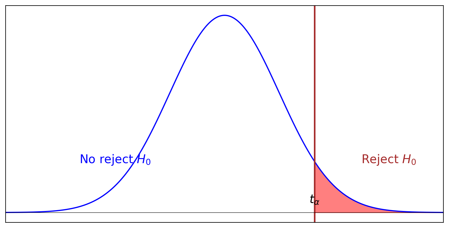
import numpy as np
import matplotlib.pyplot as plt
from scipy.stats import norm

# Generate x values
x = np.linspace(-4, 4, 1000)
# Generate y values for the normal distribution
y = norm.pdf(x, 0, 1)

# Set up the plot
plt.figure(figsize=(10, 5))

# Plot the normal distribution curve
plt.plot(x, y, color='blue')

# Shade the rejection region
x_fill = np.linspace(norm.ppf(0.95), 4, 100)
y_fill = norm.pdf(x_fill, 0, 1)
plt.fill_between(x_fill, 0, y_fill, color='red', alpha=0.5)

# Add a vertical line for the critical value
plt.axvline(norm.ppf(0.95), color='brown', linestyle='-', linewidth=2)

# Add text for the regions
plt.text(-2, 0.1, r"$\mathrm{No\  reject}\ H_0$", fontsize=15, color='blue', rotation=0, ha='center')
plt.text(3, 0.1, r"$\mathrm{Reject}\ H_0$", fontsize=15, color='brown', rotation=0, ha='center')

# Add text for the critical value
plt.text(norm.ppf(0.95), 0.02, r'$t_\alpha$', fontsize=15, color='black', ha='center')

# Remove y-axis
plt.gca().axes.get_yaxis().set_visible(False)
# Remove x-axis
plt.gca().axes.get_xaxis().set_visible(False)
# Add horizontal line
plt.axhline(0, color='black',linewidth=0.5)

# Set x-axis limits
plt.xlim(-4, 4)

# Set labels
plt.xlabel('')
plt.ylabel('')

# Show plot
plt.show()

Now, we can define the p-value as the smallest alpha threshold at which we will reject the test(T>\(t_{obs}\)). In other words, the p-value is the probability of observing an extreme value as extreme as the observed value.

So for a given alpha threshold, if the p-value is less than the alpha threshold, we reject the null hypothesis. If the p-value is greater than the alpha threshold, we don’t reject the null hypothesis.

Here, we have two scenarios to compute the p-value. First, you might know the distribution of the test statistic, or you might not know the distribution of the test statistic. It is easier to compute the p-value when you know the distribution of the test statistic. Here we will assume that you don’t know the distribution of the test statistic.

1.1 The p-value under a unknown distribution of the test statistic using the bootstrap method.

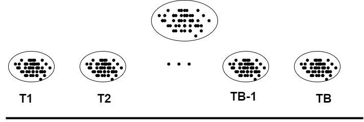
The bootstrap method is a resampling with replacement method that allows us to estimate the distribution of the test statistic. The idea is to resample with replacement the data B times and compute the test statistic for each resample(The length of resample data is smaller than the lenght of the data). The distribution of the test statistic is then the distribution of the B test statistics (T1, T2, …, TB).

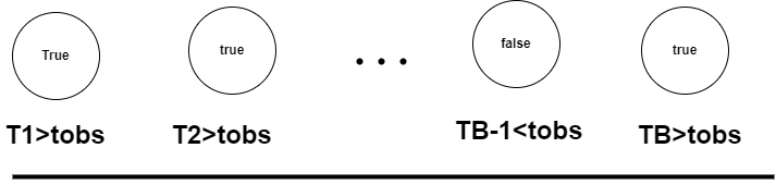
The p-value is then the proportion of the test statistics that are greater than the observed value. In other words, you compare the observed value to the distribution of the test statistic. If the test statistic is greater than the observed value, you reject the null hypothesis(you note true) and if the test statistic is less than the observed value, you don’t reject the null hypothesis(you note false).

p-value

The p-value is then the proportion of the true values :

\[ Pvalue = \frac{1}{B} \sum_{i=1}^{B} \mathbb{1}(T_i > t_{obs}) \]

where \(\mathbb{1}(T_i > t_{obs})\) is the indicator function that returns 1 if the test statistic is greater than the observed value and 0 otherwise.

Algorithm to compute the p-value under the bootstrap method

• Variables :

  • \(x_1, ..., x_n\) : the observations
  • \(t_{obs}\) : the observed value of the test statistic
  • B : the number of bootstrap samples

• Begin :

  • For b in 1 to B :

    • Sample with replacement m observations from \(x_1, ..., x_n\) to get \(x_1^b, ..., x_n^b\)
    • Compute the test statistic \(T_b\) on the bootstrap sample \(x_1^b, ..., x_n^b\)

  • Compute the p-value : \(pvalue = \frac{1}{B} \sum_{i=1}^{B} \mathbb{1}(T_i > t_{obs})\)

1.2 Implementation of the p-value under the bootstrap method with python

Now, let’s implement the p-value under the bootstrap method with python. We need to define a function that takes the observations, the function to compute the test statistic, and the number of bootstrap samples as input and returns the p-value.

def bootstrap_p_value(x ,fun, B):
    """
    Compute the p-value under the bootstrap method

    Parameters
    ----------
    x : array-like
        Observations
    fun : function
        Function to compute the test statistic
    B : int, optional
        Number of bootstrap samples, by default 1000

    Returns : float
        The p-value
    """
    n = len(x)
    
    # Compute the observed value of the test statistic
    t_obs = fun(x)

    # Resample the data B times
    t = np.zeros(B)
    for b in range(B):
        x_b = np.random.choice(x, n, replace=True)
        t[b] = fun(x_b)

    # Compute the p-value
    p_value = np.mean(t > t_obs)

    return p_value,x_b

Let’s test the function with an example. Suppose you have the following observations and you want to test if the mean of the observations is equal to 0. The test statistic is the empirical mean. We assume that the observations are drawn from a normal distribution with mean 0 and standard deviation 1 with 100 observations.

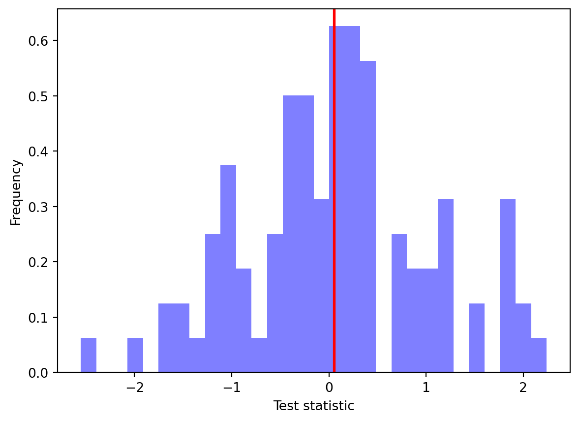
import matplotlib.pyplot as plt

# Set the seed for reproducibility
np.random.seed(0)

# Generate the observations

x = np.random.normal(0, 1, 100)

# Define the function to compute the test statistic
fun = np.mean
B = 9999
# plot the distribution of the test statistic x_b and print the p-value
p_value,x_b = bootstrap_p_value(x, fun, B)

print(f"The p-value is : {p_value}")

The p-value is : 0.49904990499049906

The p-value is 0.5, so in the threshold of 0.05, we don’t reject the null hypothesis.

# Plot the distribution of the test statistic not the histogram of the test statistic

plt.hist(x_b, bins=30, color='blue', alpha=0.5, density=True)
plt.axvline(np.mean(x_b), color='red', linestyle='-', linewidth=2)
plt.xlabel('Test statistic')
plt.ylabel('Frequency')
plt.show()

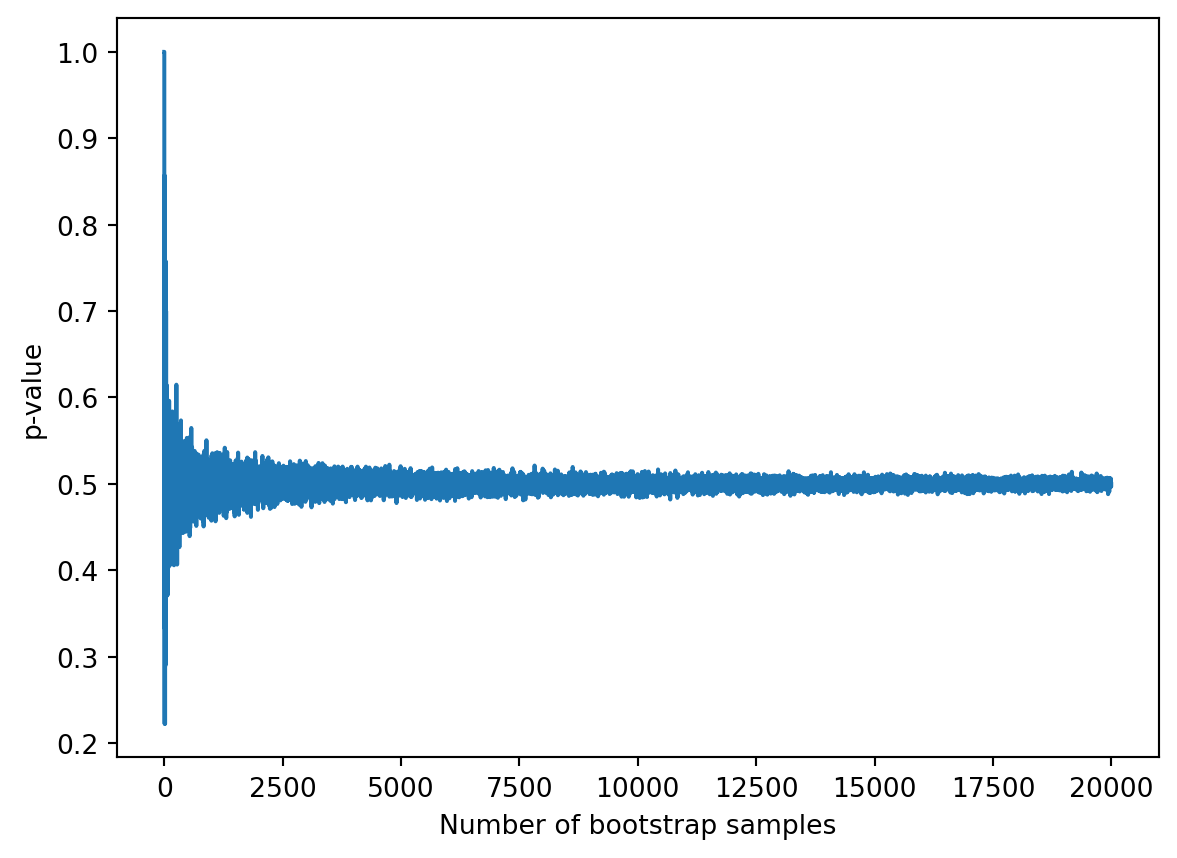
Now we can plot the ergodic mean(p-value) in order to see the convergence of the p-value.

p_values = []
for b in range(1,20000):
    p_value,_ = bootstrap_p_value(x, fun, b)
    p_values.append(p_value)
plt.plot(p_values)
plt.xlabel('Number of bootstrap samples')
plt.ylabel('p-value')
plt.show()

we can notice that the p-value converges to 0.5. This is because the observations are drawn from a normal distribution with mean 0 and standard deviation 1 when B is large enough (B>5000).

Boostrapp method is a powerful method to estimate the distribution of the test statistic when you don’t know the distribution of the test statistic. However, the bootstrap method is computationally expensive because you need to resample the data B times. In addition, the bootstrap method is not always accurate, especially when the sample size is small.