import random
import matplotlib.pyplot as plt
# Simulation de la loi uniforme sur [0, 1]
= 1000
n = [random.random() for i in range(n)]
u
# Représentation graphique
'o', label="Loi uniforme sur [0, 1]")
plt.plot(u, "Simulation de la loi uniforme sur [0, 1]")
plt.title( plt.show()
Simulation of a real and continuous random variable
Introduction
In the context of a project on copula theory, I realized that simulating random variables is not as simple as it seems. I have therefore decided to delve into the subject. In this paper, we will focus on the simulation of a real and continuous random variable X. We will use the strengths of the Python language to empirically address (with observed data) the distribution of a random variable, the law of large numbers, and the central limit theorem. I will be inspired by the book “The R Software: Mastering the Language - Performing Statistical Analyses” by Pierre Lafaye de Micheaux, Rémy Drouilhet and Benoit Liquet. I think this book is very interesting for any beginner in statistics and programming. It is very well written and very pedagogical. I highly recommend it.
The foundation of simulation: the uniform distribution on [0, 1]
I have often wondered how computers generate random numbers, and another question that bothered me was how to generate random numbers that follow a given distribution. This question is easy, you’ll see that it all comes down to the uniform distribution. And knowing how to simulate a uniform distribution will allow you to simulate any random variable distribution for which you know the cumulative distribution function. Let me explain why.
The uniform distribution is a continuous probability distribution on the interval . It is defined by the following cumulative distribution function: \(F(x) = x\) if \(x \in [0, 1]\) and \(F(x) = 0\) if \(x < 0\) et \(F(x) = 1\) if \(x > 1\). The probability density is given by \(f(x) = 1\) if \(x \in [0, 1]\) and \(f(x) = 0\) otherwise. Furthermore, the cumulative distribution function is increasing and continuous.
Now, let’s consider a real continuous random variable X, that is, one defined on a measurable space \((\Omega, \mathcal{F}, P)\) with a real-valued cumulative distribution function F defined by : \[F(x) = P(X \leq x)\]
An important result in simulation is that the random variable F(X) follows a uniform distribution. Indeed, we have: \[P(F(X) \leq x) = P(X \leq F^{-1}(x)) = F(F^{-1}(x)) = x\]
This means that we can write \(F(X) = U\), equivalent to \(X = F^(-1)(U)\), where U follows a uniform distribution on . This means that if we know how to simulate a uniform distribution, we can simulate any random variable distribution. This is what we will do in the following.
Simulation of the uniform distribution on [0, 1]
To simulate a uniform distribution on , we will use the random
function from the Python random
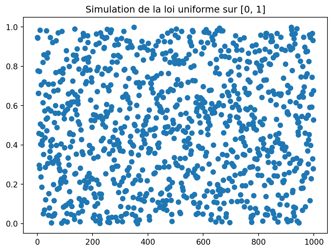
module. This function generates random numbers following a uniform distribution on . We will generate 1000 random numbers following a uniform distribution on and represent them graphically.
We notice that the values are uniformly distributed on the interval . This means that the simulation is correct. We will now simulate an exponential distribution with parameter \(\lambda = 1\). Its cumulative distribution function is given by: \[F(x) = 1 - e^{-x}\] And its inverse function is given by: \[F^{-1}(x) = -\ln(1-x)\]
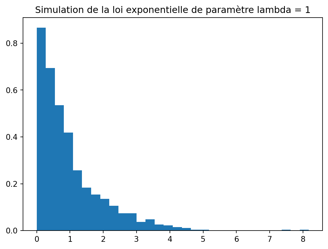
We will simulate 1000 values of the exponential distribution with parameter \(\lambda = 1\) and represent them graphically.
import numpy as np
# Simulation de la loi exponentielle de paramètre lambda = 1
= [-np.log(1 - u[i]) for i in range(n)]
x
# Représentation graphique
=30, density=True, label="Loi exponentielle de paramètre lambda = 1")
plt.hist(x, bins"Simulation de la loi exponentielle de paramètre lambda = 1")
plt.title( plt.show()
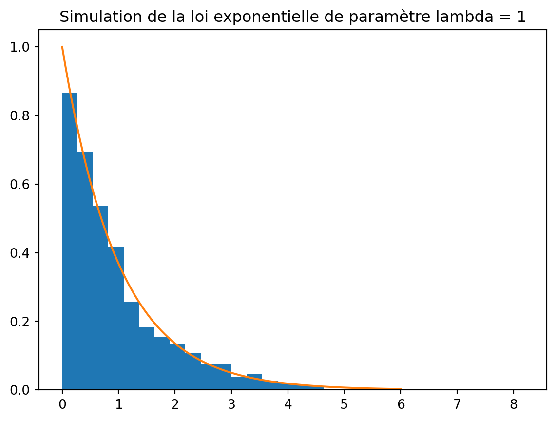
We notice that the values are well distributed according to an exponential distribution with parameter \(\lambda = 1\). We will superimpose the density of an exponential distribution with parameter equal to 1 to show how perfect our simulation is.
import scipy.stats as stats
# Représentation graphique
=30, density=True, label="Loi exponentielle de paramètre lambda = 1")
plt.hist(x, bins0, 6, 100), stats.expon.pdf(np.linspace(0, 6, 100)), label="Densité de la loi exponentielle de paramètre lambda = 1")
plt.plot(np.linspace("Simulation de la loi exponentielle de paramètre lambda = 1")
plt.title( plt.show()
Thank you for reading. If you have any questions or comments, please do not hesitate to contact me. I will be happy to answer you.