Climate Risk Measures

Climate Risk
Author

Jumbong Junior

Published

May 10, 2024

1 Introduction

This paper is for those who believe in the critical importance of sustainability and a future with low carbon emissions. That’s why I published it on Medium. I hope that it will be helpful to those who are interested in the integration of climate risk into traditional business models. When I was working on my final year project, I was looking for a way to integrate climate risk into asset allocation models. As I reviewed the literature, I read many articles.I think it’s important to understand climate risk metrics before making a complicated decision model.

When working with a portfolio of a n asset, The concern of investor is to determine the weight \(w=(w_1,...w_n)\) of each asset in the portfolio. The investor wants to know how much invest in each asset. Answering this question is the same as determining what weight assign to each asset.

The traditional portfolio optimization responds to this question. It requires input data such as the vector of expected returns \((\mu_1,...,\mu_n)\) of asset, the vector \(\sigma\) of asset volatilities and the correlation matrix \(\rho\) of asset returns. We can then compute the first and second moment of the stochastics portfolio return. In particular, the portfolio risk corresponds to the portfolio volatility \(\sigma(x)\). To be more precise, using the parameters \(\sigma\) and \(\rho\), we can compute the portfolio covariance matrix \(\Sigma\), which is defined as follows: \(\Sigma_{ij} = \sigma_i \sigma_j \rho_{ij}\). The first moment is equal to the expected return of the portfolio \(\mu(x) = \sum_{i=1}^{n} w_i \mu_i\) While the second is equal to the variance of the portfolio returns \(\sigma(x) = \sqrt{\sum_{i=1}^{n} \sum_{j=1}^{n} w_i w_j \Sigma_{ij}}\).

When introducing climate-related risk, we have to define another measure \(C(w_1,...w_n)\) that assesses the risk of climate change. Let consider a climate metrics \(C_i\) of associated with asset \(i\). The nature of the climate risk is then different from the volatility risk measure since the latter satisfy the sod additivity property : \[\sigma(w) <= \sum_{i=1}^{n} w_i \sigma_i\]

Even if \(C(w)\) is a convex risk measure, it is an abuse of language, because there is no way to diversify the climate risk: \[C(w) \not < \sum_{i=1}^{n} w_i C_i\]

Therefore, \(C(w)\) play more the rule of an expected loss than a risk measure. In this paper, we will present some climate risk measures. First, we will present carbon footprint and carbon intensity.
2 Carbon Footprint

Carbon footprint is an indicator of the amount of greenhouse gas(GHG) emissions caused by human activities. Greenhouse gases absorb and emit radiation energy emitted by the Earth once the sun has warmed its surface, causing the greenhouse effect. The most common greenhouse gases are carbon dioxide (CO2), methane (CH4), and nitrous oxide (N2O). It’s important to remind that the greenhouse effect Was crucial for the development of human life on Earth. Without it, the average temperature of the Earth would be -18°C. With the greenhouse effect, the current temperature of Earth’s surface is about +15°C. However, the increase in greenhouse gas emissions due to human activities has led to an increase in the greenhouse effect, which has caused global warming.

Carbon footprint is expressed in CO2 equivalent (CO\(_2\)e), which is a term for describing different GHGs in a common unit. In another word, a quantity of GHG is express as C0\(_2\)e By multiplying the GHG amount by its global warming potential(GWP).The GWP of a gas is the amount of a gas that would cause the same amount of warming as a CO2 over a specific time period. For example, the IPCC’s \(4^{th}\) assessment report has used the following rules : 1 kg of methane corresponds to 25 kg of CO_\(2\) and 1 kg of nitrous oxide corresponds to 298 kg of CO\(_2\).

This indicator allows to properly compare companies in the same sector or have the same characteristics. If the size of companies are not the same, it is better to use normalize indicator like carbon intensity.

To provide a common measure That can be used by all companies and to limit bias. The Greenhouse gas protocol has defined three scopes of carbon emissions.

### The three scopes of carbon emissions

  • Scope 1 refers to direct emissions from sources that are owned or controlled by the company. For example, we can mention emissions from combustion in owned or controlled boilers, furnaces, vehicles, and air conditioning systems.

  • Scope 2 denotes indirect emissions from the generation of purchased electricity, steam, heating, and cooling consumed by the company. For example, we can mention emissions from the generation of electricity purchased and used by the company.

  • Scope 3 includes all other indirect emissions that occur in a company’s value chain. For example, we can mention emissions from the extraction and production of purchased materials and fuels, transport-related activities in vehicles not owned or controlled by the reporting entity, electricity-related activities not covered in Scope 2, outsourced activities, waste disposal, etc.

In what follows, we distinguish these three carbon emission measures by introducing the notations CE1, CE2 and CE3. Moreover, they are generally expressed in tons of carbon dioxide equivalent or tCO\(_2\)e. Now we have a tool to construt our carbon metrics

2.1 Carbon metrics

The carbon metrics that is generally used to compare entities or companies is the carbon Intensity. The carbon intensity of company i with respect to scope j is defined as the ratio of the carbon emissions of scope j to the activity of the company. The carbon intensity of company i with respect to scope j is defined as follows:

\[CI_{ij} = \frac{CE_{ij}}{Y_i}\]

where \(CE_{ij}\) is the carbon emissions of company i with respect to scope j and \(Y_i\) is the activity of company i. The carbon intensity of company i is then defined as the sum of the carbon intensity of each scope:

where Y is an indicator measuring the activity of the company. For example, it can be the revenue, the number of employees, the number of products sold, etc. To apply this, we will you the data of the company. The data below comes from Trucost reporting year 2019.

import pandas as pd
carbon_footprint = pd.read_csv('carbon_footprint.csv', index_col=0)
carbon_footprint.head()
Company Emission Scope 1 Emission Scope 2 Emission Scope 3 Revenue
0 Alphabet 74462.0 5116949 7166240 161857
1 Amazon 5760000.0 5500000 20054722 280522
2 Apple 50463.0 862127 27618943 260174
3 BP 49199999.0 5200000 103840194 276850
4 Danone 722122.0 944877 28969780 28308

To compute the carbon intensity, we can first compute the carbon intensity for each scope and then sum them up.

carbon_footprint['CE1'] = carbon_footprint['Emission Scope 1'] / carbon_footprint['Revenue']
carbon_footprint['CE2'] = carbon_footprint['Emission Scope 2'] / carbon_footprint['Revenue']
carbon_footprint['CE3'] = carbon_footprint['Emission Scope 3'] / carbon_footprint['Revenue']
carbon_footprint['CI'] = carbon_footprint['CE1'] + carbon_footprint['CE2'] + carbon_footprint['CE3']
carbon_footprint.head()
Company Emission Scope 1 Emission Scope 2 Emission Scope 3 Revenue CE1 CE2 CE3 CI
0 Alphabet 74462.0 5116949 7166240 161857 0.460048 31.614011 44.275132 76.349191
1 Amazon 5760000.0 5500000 20054722 280522 20.533149 19.606305 71.490728 111.630182
2 Apple 50463.0 862127 27618943 260174 0.193959 3.313655 106.155661 109.663275
3 BP 49199999.0 5200000 103840194 276850 177.713560 18.782734 375.077457 571.573751
4 Danone 722122.0 944877 28969780 28308 25.509467 33.378444 1023.377844 1082.265755

One advantage of carbon intensity is that it reduces the skewness of the data.

## Skewness of the data
carbon_footprint[['Emission Scope 1', 'Emission Scope 2', 'Emission Scope 3', 'CI']].skew()
Emission Scope 1    2.165456
Emission Scope 2    0.054302
Emission Scope 3    1.243665
CI                  1.559668
dtype: float64
## Skewness of the data
carbon_footprint[['CE1', 'CE2', 'CE3', 'CI']].skew()
CE1    2.087192
CE2    0.813709
CE3    1.997709
CI     1.559668
dtype: float64

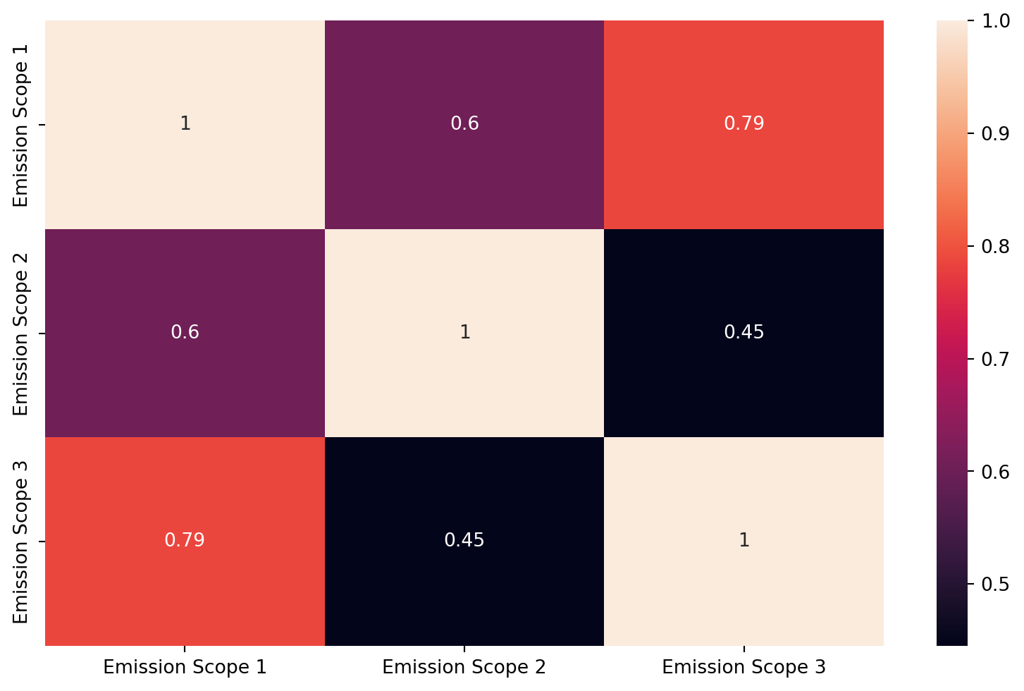
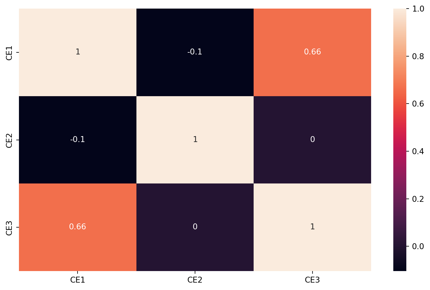
Let’s now visualize the spearman correlation between the several carbon metrics.

import seaborn as sns
import matplotlib.pyplot as plt
plt.figure(figsize=(10, 6))
sns.heatmap(carbon_footprint[['Emission Scope 1', 'Emission Scope 2', 'Emission Scope 3']].corr(), annot=True)
plt.show()

import seaborn as sns
import matplotlib.pyplot as plt
plt.figure(figsize=(10, 6))
sns.heatmap(carbon_footprint[['CE1', 'CE2', 'CE3']].corr(), annot=True)
plt.show()

We notice that carbon emissions are highly correlated that carbon intensity because of the economic size effect (\(33\%\) in average vs \(23\%\) in average). Now let’s visualize the rank correlation between the carbon metrics.

plt.figure(figsize=(10, 6))
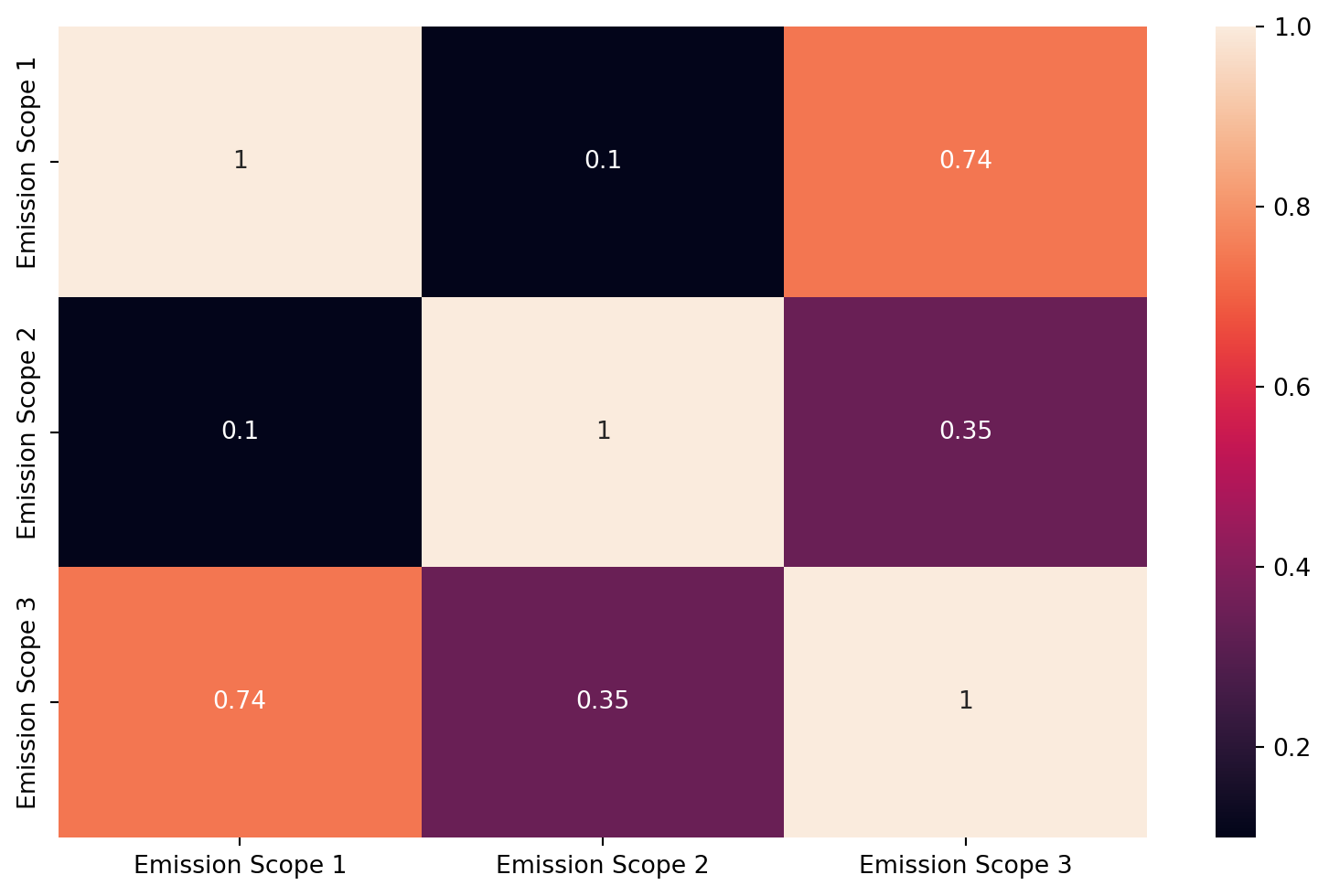
sns.heatmap(carbon_footprint[['Emission Scope 1', 'Emission Scope 2', 'Emission Scope 3']].corr(method='spearman'), annot=True)
plt.show()

plt.figure(figsize=(10, 6))
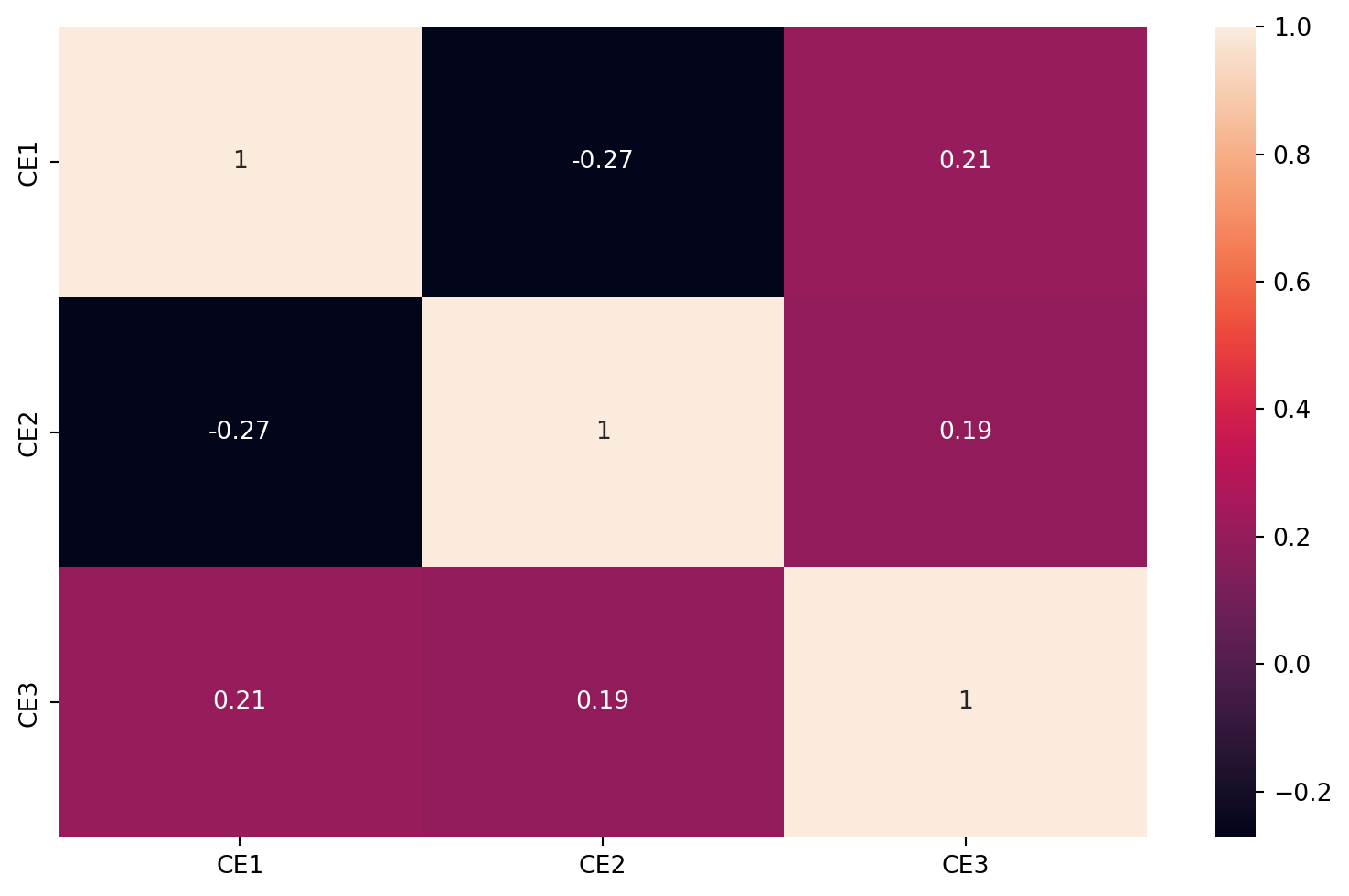
sns.heatmap(carbon_footprint[['CE1', 'CE2', 'CE3']].corr(method='spearman'), annot=True)
plt.show()

We notice that rank correlation between carbon emissions is higher than the rank correlation between carbon intensity, and rank correlation are very lower for all carbon intensity.

Let’s finish this section with the additivity property of carbon intensity.

2.2 Additivity property of carbon intensity

For a company i, the carbon intensity is additive. For example, the carbon intensity for a company i with respect to scope 1,2 and 3 is defined as follows: \[ \begin{align} CL_{i,1+2+3} &= \frac{CE_{i,1} + CE_{i,2} + CE_{i,3}}{Y_i} \\ &= CI_{i,1} + CI_{i,2} + CI_{i,3} \end{align} \]

However, this property is not satisfied when we consider the carbon intensity of a portfolio of companies. Let us consider a portfolio of weights \(w=(w_1,...,w_n)\) investing in n assets(stock, bond, etc). Its carbon emissions are defined as follows:

\[ CE_{j} = \sum_{i=1}^{n} \frac{W_i}{MV_i} CE_{ij} = \sum_{i=1}^{n} \bar{w_i} CE_{ij} \]

where \(MV_i\) is the market value the company i and j is the scope of carbon emissions, and \(W_i\) is the dollar amount invested in company i. \(\bar{w_i}\) is the ownership ratio:

\[ \bar{w_i} = \frac{W_i}{MV_i} \]

If you invest \((x_1,...,x_n)\) where \(x_i\) is the dollar amount invested in company i, \(x=\sum_{i=1}^{n} x_i\) is the total amount invested in the portfolio. We deduce that :

\[ \bar{w_i} = w_i \frac{x}{MV_i} \]

and:

\[ \begin{align} CE_{j} &= \sum_{i=1}^{n} w_i \frac{x}{MV_i} CE_{ij} \\ &= x \sum_{i=1}^{n} \frac{w_i}{MV_i} CE_{ij} \\ &= x \sum_{i=1}^{n} \frac{w_i Y_i}{MV_i} \frac{CE_{ij}}{Y_i} \\ \end{align} \]

This equation equation gives us an interpretation of the carbon emission as weighted average of the carbon intensity where the normalization is the market value of the company. In other words :

\[ CE_{j} = x \sum_{i=1}^{n} w_i CI_{ij}^{MV} \]

where \(CI_{ij}^{MV} =\frac{CE_{ij}}{MV_i}\) is the carbon intensity of company i with respect to scope j normalized by the market value of the company.

2.3 Be aware of mixing large capitalization and small capitalization companies.

If we assume that the equation below is true:

\[ CE_{j} = \sum_{i=1}^{n} \frac{W_i}{MV_i} CE_{ij} = \sum_{i=1}^{n} \bar{w_i} CE_{ij} \]

Then we can show that (refer to the page 8 and in appendix ix A.4.1 on page 45 on this book for more details):

\[ CI_{j}(w) = \sum_{i=1}^{n} x_i CI_{ij} \]

where the weights \(x_i\) are defined as follows:

\(x_i = \frac{w_i\frac{Y_i}{MV_i}}{\sum_{i=1}^{n} w_i\frac{Y_i}{MV_i}} = \frac{w_i SR_i}{\sum_{i=1}^{n} w_i SR_i}\)

where \(SR_i = \frac{Y_i}{MV_i}\) is the revenue-to-market value (or sales-to-price) ratio.

Now consider two issuers. The first issuer has a carbon emissions, revenue and market respectively equal to \(CE_{1,j} = 5 \times 10^6\), \(Y_1 = 2 \times 10^5\) and \(MV_1 = 10^7\). The second issuer has a carbon emissions, revenue and market respectively equal to \(CE_{2,j} = 5 \times 10^7\), \(Y_2 = 4 \times 10^6\) and \(MV_2 = 10^7\). We suppose we invest x=$10 mm to the issuers.

Let’s write utility classes to compute the carbon intensity of each issuer, the carbon emissions of the portfolio and the carbon intensity of the portfolio.

from collections.abc import Iterable
class CarbonIntensity:
    @staticmethod
    def carbon_intensity_issuer(
        __CE: Iterable[float],
        __Y: Iterable[float],

    ):

        return __CE / __Y
    @staticmethod
    def revenue_to_market(
        Y: Iterable[float],
        MV: Iterable[float]
    ):

        return Y / MV
    @staticmethod
    def carbon_emission_portfolio(
        x: Iterable[float],
        CE: Iterable[float],
        w: Iterable[float],
        MV: Iterable[float]
    ):
    
        return sum([x * w * CE / MV for x, w, CE, MV in zip(x, w, CE, MV)])
    @staticmethod
    def carbon_intensity_portfolio(
        w: Iterable[float],
        Y: Iterable[float],
        MV: Iterable[float],
        CI: Iterable[float]
    ):
        total_revenue_tomarket = sum([(w * Y) / (MV) for w, Y, MV in zip(w, Y, MV)])
        return sum([(w*Y*CI)/(total_revenue_tomarket* MV) for w, Y, CI, MV in zip(w, Y, CI, MV)])

It follows that the carbon intensity of the first issuer is equal to 25 and the carbon intensity of the second issuer is equal to 12.5. It is given by the following code:

CE1, CE2 = 5e6, 5e7
Y1, Y2 = 2e5, 4e6

CarbonIntensity.carbon_intensity_issuer(CE1, Y1), CarbonIntensity.carbon_intensity_issuer(CE2, Y2)
(25.0, 12.5)

The revenue-to-market ratio of the first issuer is equal to 0.02 and the revenue-to-market ratio of the second issuer is equal to 0.4. It is given by the following code:

MV1, MV2 = 1e7, 1e7
CarbonIntensity.revenue_to_market(Y1, MV1), CarbonIntensity.revenue_to_market(Y2, MV2)
(0.02, 0.4)

Now, let’s compute the carbon emissions of the portfolio and the carbon intensity of the portfolio. If the weights of the first issuer is \(w_1\) and the weights of the second issuer is \(w_2\), The revenue that will be use to compute the carbon intensity of the portfolio is equal: \(Y = w_1 \times Y_1 + w_2 \times Y_2\) The weights \(x_1\) and \(x_2\) are given by the following code:

weights = {
    'w1': ["0%", "10%", "20%", "30%", "50%", "70%", "80%", "90%", "100%"],
    'w2': ["100%", "90%", "80%", "70%", "50%", "30%", "20%", "10%", "0%"]}
weights['w1'] = [float(w.replace('%', '')) / 100 for w in weights['w1']]
weights['w2'] = [float(w.replace('%', '')) / 100 for w in weights['w2']]

First we Compute the revenue to compute the carbon intensity of the portfolio :

carbon_intensity_portfolio_approach = pd.DataFrame()
carbon_intensity_portfolio_approach['w1'] = weights['w1']
carbon_intensity_portfolio_approach['w2'] = weights['w2']
carbon_intensity_portfolio_approach['Y *10^6'] = carbon_intensity_portfolio_approach['w1'] * Y1/1e6 + carbon_intensity_portfolio_approach['w2'] * Y2/1e6
carbon_intensity_portfolio_approach
w1 w2 Y *10^6
0 0.0 1.0 4.00
1 0.1 0.9 3.62
2 0.2 0.8 3.24
3 0.3 0.7 2.86
4 0.5 0.5 2.10
5 0.7 0.3 1.34
6 0.8 0.2 0.96
7 0.9 0.1 0.58
8 1.0 0.0 0.20

Then we compute the carbon emissions of the portfolio and the carbon intensity of the portfolio:

carbon_intensity_portfolio_approach['CE*10^6'] = CarbonIntensity.carbon_emission_portfolio(
    x=[10e6, 10e6],
    CE=[CE1, CE2],
    w=[carbon_intensity_portfolio_approach['w1'], carbon_intensity_portfolio_approach['w2']],
    MV=[MV1, MV2]
)/1e6
carbon_intensity_portfolio_approach
w1 w2 Y *10^6 CE*10^6
0 0.0 1.0 4.00 50.0
1 0.1 0.9 3.62 45.5
2 0.2 0.8 3.24 41.0
3 0.3 0.7 2.86 36.5
4 0.5 0.5 2.10 27.5
5 0.7 0.3 1.34 18.5
6 0.8 0.2 0.96 14.0
7 0.9 0.1 0.58 9.5
8 1.0 0.0 0.20 5.0

Then we compute the carbon intensity of the portfolio. To do this, we need the carbon emissions of the portfolio and the revenue of the portfolio. The carbon intensity of the portfolio is given by the following code:

carbon_intensity_portfolio_approach['CI/Y'] = carbon_intensity_portfolio_approach['CE*10^6'] / carbon_intensity_portfolio_approach['Y *10^6']
carbon_intensity_portfolio_approach 
w1 w2 Y *10^6 CE*10^6 CI/Y
0 0.0 1.0 4.00 50.0 12.500000
1 0.1 0.9 3.62 45.5 12.569061
2 0.2 0.8 3.24 41.0 12.654321
3 0.3 0.7 2.86 36.5 12.762238
4 0.5 0.5 2.10 27.5 13.095238
5 0.7 0.3 1.34 18.5 13.805970
6 0.8 0.2 0.96 14.0 14.583333
7 0.9 0.1 0.58 9.5 16.379310
8 1.0 0.0 0.20 5.0 25.000000

we finish this section by computing the carbon intensity of the portfolio using the weights defined by: \(x_i = \frac{w_i\frac{Y_i}{MV_i}}{\sum_{i=1}^{n} w_i\frac{Y_i}{MV_i}} = \frac{w_i SR_i}{\sum_{i=1}^{n} w_i SR_i}\)

carbon_intensity_portfolio_approach[‘CI’] = CarbonIntensity.carbon_intensity_portfolio( w=[carbon_intensity_portfolio_approach[‘w1’], carbon_intensity_portfolio_approach[‘w2’]], Y=[Y1, Y2], MV=[MV1, MV2], CI=[CarbonIntensity.carbon_intensity_issuer(CE1, Y1), CarbonIntensity.carbon_intensity_issuer(CE2, Y2)] ) carbon_intensity_portfolio_approach