Resampling methods : Permutation Test

Author

Jumbong Junior

Introduction

Resampling methods are a key part of statistical inference. It is important to understand them in order to have accurate estimates, validate models, and dealt with the uncertainty of the data. Indeed, the resampling methods mesure the variability of statistics by using subsamples from the original data. There are least four resampling methods: bootstrap, jackknife, permutation test, and cross-validation :

Resampling method	Applications	Type of resampling
Efron’s bootstrap	Bias, variance, confidence intervals, hypothesis testing	With replacement
Permutation test	Hypothesis testing	Without replacement
Jackknife	Bias, variance, confidence intervals	Leave-one-out
Cross-validation	Model selection, validation	Leave-p-out

This document will focus on the permutation test.

General framework of the hypothesis test

The goal of statistics is to learn about a population by studying a sample. Often, we don’t know the process that produced the sample. Mathematically, the sample is a random variable.

Let \(X = (X_1, X_2, \ldots, X_n)\) be a sample of size \(n\) drawn from a population or a probability distribution \(P\).

A hypothesis is a declarative statement about the population or the probability distribution. A hypothesis test involves two complementary hypotheses :

The null hypothesis \(H_0\) : “\(P \in \mathcal{P}_0\)” where \(\mathcal{P}_0\) is a set of probability distributions.
The alternative hypothesis \(H_1\) : “\(P \notin \mathcal{P}_0\)”.

A test \(\phi\) is a decision procedure between \(H_0\) and \(H_1\), given the sample \(X\). \[ \phi(x) = \begin{cases} 1 & \text{reject} H_0 \\ 0 & \text{It is not reject} H_0 \end{cases} \]

A test \(\phi\) is defined using a real-valued test statistic \(T(X)\) :

\(\phi(x) = \mathbb{1}_{\{T(x) > t_{\alpha}\}}\) where \(t_{\alpha}\) is the critical value of the test at level \(\alpha\). \(H_0\) is rejected when \(T(x) > t_{\alpha}\).
\(\sup_{P \in \mathcal{P}_0} \mathbb{E}_P \{\phi\} \leq \alpha : \text{ The law of } T \text{ under } H_0 \text{ is known}\).

The p-value of a test is the smallest level \(\alpha\) at which the null hypothesis is rejected : \[ p(x) = \inf \{ \alpha : T(x) > t_{\alpha} \} \]

To construct a test, it is necessary to know the distribution or the law of the test statistic under the null hypothesis in other to compute :

The critical value \(t_{\alpha}\).
The p-value \(p(x)\).

Motivation of the permutation test

In pratice, the law of the test statistic T is often approximated asymptotically, or requires verifying parametric assumptions that are hard to justify (eg. normality, homoscedasticity, etc.).

The permutation test is a non-parametric test. It can be used :

When the size of the sample is small to approximate the law of the test statistic.
When parametric test is not valid.

General framework of the permutation test

Principle : Working on the observed data to avoid having to assume a specific distribution for the observed sample.

General Principle

The statistical Model : \(X \sim P, P \in \mathcal{P}\). \(P\) is a probability defined on \(\mathbb{R}^N\) and \(\mathcal{P}\) is a set of probability distributions on \(\mathbb{R}^N\).

The hypothesis test : \(H_0 : P \in \mathcal{P}_0\) vs \(H_1 : P \notin \mathcal{P}_0\). \(\mathcal{P}_0\) is a subset of \(\mathcal{P}\).

Group of Transformations : \(G\) has the size \(|G| = M\). \(G\) has an idendity element \(e\). The operation inside \(G\) is associative : \(g_1, g_2 \in G \Rightarrow g_1 \cdot g_2 \in G\). For each \(g \in G\), there is an inverse element \(g^{-1}\) such that \(g \cdot g^{-1} = g^{-1} \cdot g = e\).

\(G\) acts on \(\mathbb{R}^N\) : \(g \in G, x \in \mathbb{R}^N \Rightarrow g \cdot x \in \mathbb{R}^N\). where \(e \cdot x = x\) and \(g_1 \cdot (g_2 \cdot x) = (g_1 g_2) \cdot x\)

Echangeability Assumption

Under \(H_0\) (\(P \in \mathcal{P}_0\)): for every \(g \in G\), \(\mathcal{L}_P(g \cdot X) = \mathcal{L}_P(X)\).

Permutation Test : The permutation test is a test that uses the exchangeability assumption to construct a test.

Let’s define the decision function \(\phi\) and the p-value \(p\) of the permutation test :

Permutation Test with Level \(\leq \alpha\)

\[ \phi(X) = \mathbb{1}_{\{T(X) >T^{(\lceil M(1-\alpha) \rceil)}\}} \] where \(T^{(\lceil M(1-\alpha) \rceil)}\) is the \(\lceil M(1-\alpha) \rceil\)-th order statistic of the test statistic \(T(g \cdot X)\) for \(g \in G\).

The p-value of the permutation test is : \[ p(X) = \frac{1}{M} \sum_{g \in G} \mathbb{1}_{\{T(g \cdot X) > T(X)\}} \]

Application of the permutation test

The permutation test has many applications in statistics :

Symmetry test : The permutation test can be used to test the symmetry of a distribution. An example is the Wilcoxon sign-rank test for paired samples.
Independence test : which help assess the effect of one variable on another. An example is the Spearman test.
Comparison of two samples : The permutation test can be used to compare the distribution of two samples. For example to assess if two samples have the same law.

Symmetry test

Statistical Model : \(X = (X_1, X_2, \ldots, X_n)\overset{i.i.d}{\sim} F\) where \(F\) is a Cumulative Distribution Function (CDF) defined on \(\mathbb{R}\). \(X = (X_1, \dots, X_n) \in \mathbb{R}^n\)

The hypothesis test : \(H_0 : F \text{ is symmetric around } 0\) vs \(H_1 : F \text{ is not symmetric around } 0\).

The transformation group : \(G = \{-1, 1\}^n\). with cardinality \(|G| = 2^n\).

Exchangeability Assumption

Under \(H_0\) (\(F\) is symmetric around 0) : for every \(g \in G\), \(\mathcal{L}_F(g \cdot X) = \mathcal{L}_F(X)\).

Test statistic : The test statistic can be defined by :

T(X) = |\(\overline{X}\)| where \(\overline{X} = \frac{1}{n} \sum_{i=1}^n X_i\).
\(T(X) = \sum_{i=1}^n R_i sign(X_i)\) where \(R_i\) is the rank of \(|X_i|\) in \(|X_1|, |X_2|, \ldots, |X_n|\).

Algo : Symmetry test by permutation test (Monte Carlo)

Variable :

B : 999,999 such that (B+1)\(\alpha\) is an integer.

Begin :

for b = 1 to B do:

Generate \(g^b \sim \mathcal{U}(G)\)
Compute \(T^b = T(g^b \cdot X)\).

end for.

Return the p-value \(p(X) = \frac{1}{B} \sum_{b=1}^B \mathbb{1}_{\{T^b > T(X)\}}\)

end

The code below is an implementation of the permutation test for the symmetry test.

import numpy as np


# Inputs : x (array) or (list) : sample.
#func : function : statistic function.
#nsamp : int : number of samples.
# Outputs : dictionnary : statistic, sample_perm, p-value.

def symmetry_perm(x, func=np.mean, nsamp =9999):
    x = np.asarray(x)
    n = x.shape[0]

    tobs = func(x)
    # Generate nsamp samples sign permutation
    eps = np.random.choice([-1, 1], size=(nsamp, n), replace=True)
    # Compute the test statistic for each sample
    permuted = eps * x

    try:
        tperm = func(permuted, axis=1)
    except TypeError:
        tperm = np.apply_along_axis(func, 1, permuted)
    # Compute the p-value

    count = np.sum(np.abs(tperm) >= np.abs(tobs))
    p = (count + 1) / (nsamp + 1)
    return {"statistic": tobs, "sample_perm": tperm, "p-value": p}

Let’s apply the symmetry test to a central normal distribution.

#np.random.seed(42)

n = 100
x = np.random.normal(0, 1, n)

res = symmetry_perm(x, func=np.mean, nsamp=9999)

print(f"Statistic : {res['statistic']}," 
      f" p-value : {res['p-value']}")

Statistic : 0.016915530800782546, p-value : 0.8739

Distribution of the mean and the ergodic mean p-values.

B = 6000
# P value for a range of nsamp from 1 to B
p_values = [symmetry_perm(x, func=np.mean, nsamp=i)["p-value"] for i in np.arange(1, B)]


import matplotlib.pyplot as plt
import seaborn as sns   

fig, axes = plt.subplots(1, 2, figsize=(8, 3))

## 🟢 Histogram: Distribution of Test Statistic
sns.histplot(res['sample_perm'], ax=axes[0], kde=True, color='#1f77b4', alpha=0.7)
axes[0].axvline(res['statistic'], color='red', linestyle='--', linewidth=2, label='Observed Statistic')
axes[0].set_title('Distribution of the Test Statistic', fontsize=14, fontweight='bold')
axes[0].set_xlabel('Test Statistic', fontsize=12)
axes[0].set_ylabel('Frequency', fontsize=12)
axes[0].legend(fontsize=12)
# No grid for better readability
axes[0].grid(False)

## 🔵 Line Plot: Ergodic Mean of the P-value
axes[1].plot(np.arange(1, B), p_values, color='#ff7f0e', linewidth=2)
axes[1].axhline(np.mean(p_values), color='black', linestyle='--', linewidth=2, label='Mean p-value')
axes[1].set_title('Ergodic Mean of the P-value', fontsize=14, fontweight='bold')
axes[1].set_xlabel('Iterations', fontsize=12)
axes[1].set_ylabel('P-value', fontsize=12)
axes[1].legend(fontsize=12)
axes[1].grid(False)
# Annotation for Mean P-value
axes[1].text(0.6 * B, np.mean(p_values), f"Mean p-value: {np.mean(p_values):.4f}",
             fontsize=12, color='black', fontweight='bold')

# Improve layout
plt.tight_layout()

# Show the plot
plt.show()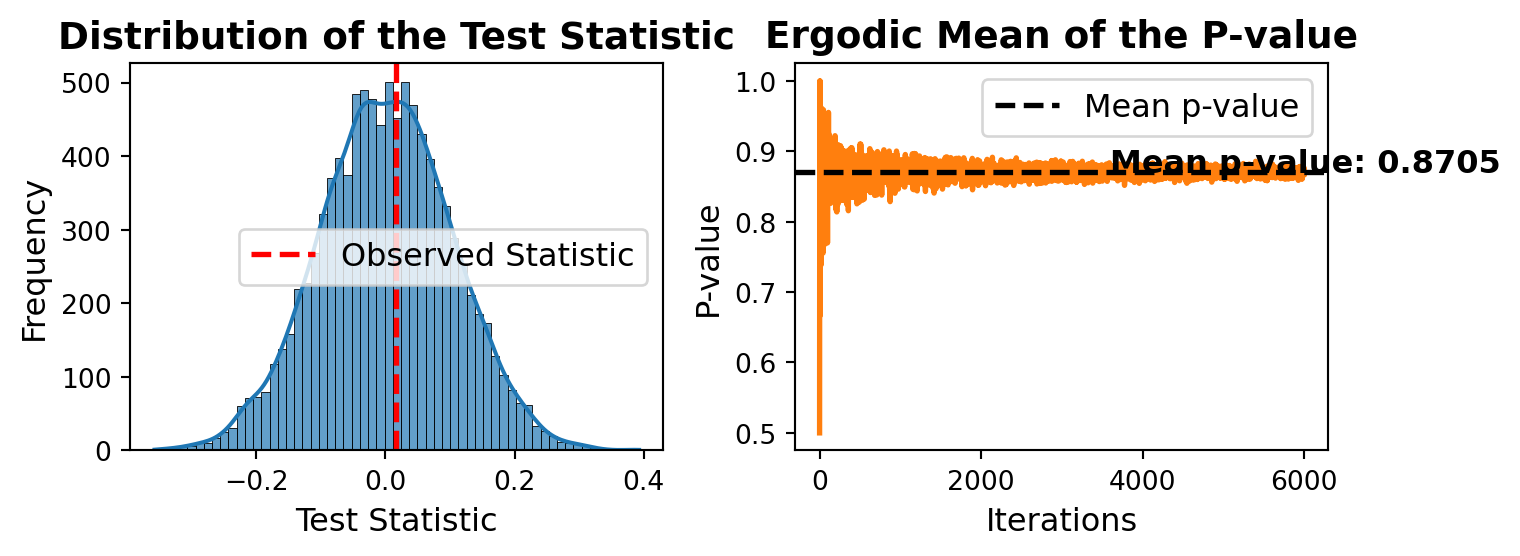

Symmetry test : Wilcoxon sign-rank test

One of the most popular permutation tests is the Wilcoxon sign-rank test. It allows to test for example if two paired samples come from the same distribution. To accomplish this, the Wilcoxon sign-rank test assess if the difference between the two samples is symmetric around 0.

The test statistic is defined by :

\[ T(X) = \sum_{i=1}^n R_i sign(X_i) \]

where \(R_i\) is the rank of \(|X_i|\) in \(|X_1|, |X_2|, \ldots, |X_n|\).

For the application of the Wilcoxon sign-rank test, for 10 patients, we have data on the number of hours of sleep after taking a drug and after taking a placebo. The goal is to test if the number of hours of sleep is the same after taking the drug and the placebo.

from scipy.stats import wilcoxon, PermutationMethod
import pandas as pd

treatment = np.array([6.1,7.0,8.2,7.6,6.5,8.4,6.9,6.7,7.4,5.8])
placebo  = np.array([5.2,7.9,3.9,4.7,5.3,5.4,4.2,6.1,3.8,6.3])
z = treatment - placebo
# Stat test 
statW = lambda z: (pd.Series(np.abs(z)).rank() * np.sign(z)).sum()

# Test per permutation
res = symmetry_perm(z, func=statW, nsamp=59999)

print(f"Statistic : {res['statistic']}," 
      f" p-value : {res['p-value']}")

Statistic : 45.0, p-value : 0.0199

The p-value is 0.01985 less than 0.05, we reject the null hypothesis. The number of hours of sleep is not the same after taking the drug and the placebo.

Independence test

Let’s define the framework of the independence test :

Statistical Model : \((Y_1,Z_1), (Y_2,Z_2), \ldots, (Y_n,Z_n) \overset{i.i.d}{\sim} F\) where \(F\) is a joint distribution defined on \(\mathbb{R}^2\). X = \((Y, Z) = (Y_1, Z_1), (Y_2, Z_2), \ldots, (Y_n, Z_n)\), matrix of size \(n \times 2\).

The hypothesis test : \(H_0 : F(y,z) = F_Y(y)F_Z(z)\) vs \(H_1 : F(y,z) \neq F_Y(y)F_Z(z)\). where \(F_Y\) and \(F_Z\) are the marginal distributions of \(Y\) and \(Z\).

The transformation group : G is the permutation group of size \(|G| = n!\). G acts on \(\mathbb{\textbf{M}}^{2 \times n}\) by : \[ \sigma \cdot X = \bigl((y_1, z_{\sigma(1)}), (y_2, z_{\sigma(2)}), \ldots, (y_n, z_{\sigma(n)})\bigr) \] For \(\sigma \in G\) and \(X = (Y, Z)\).

The test statistic (association measure or correlation) is defined by :

T(X) = \(\sum_{i=1}^n (Y_i - \overline{Y})(Z_i - \overline{Z})\), pearson correlation.
T(X) = \(\sum_{i=1}^n R_i(Y) R_i(Z) - \frac{4(n+1)^2}{n}\), Spearman correlation.

Algo : Independence test by permutation test (Monte Carlo)

Variable :

B : 999,999 such that (B+1)\(\alpha\) is an integer.

Begin :

for b = 1 to B do:

Generate \(\sigma^b \sim \mathcal{U}(G)\) (Transformation group)
Compute \(T^b = T(\sigma^b \cdot X)\). (law of permutation)

end for.

Return the p-value \(p(X) = \frac{1}{B+1} (\sum_{b=1}^B (\mathbb{1}_{\{T^b > T(X)\}}) + 1)\)

end

For example, We want to study the effect of the molar ratio of sebacic acid to the intrinsic viscosity of copolyster. The data is given by :

molar_ratio = np.array([1, 0.9, 0.8, 0.7, 0.6, 0.5, 0.4, 0.3])
viscosity = np.array([0.45, 0.2, 0.34, 0.58, 0.7, 0.57, 0.55, 0.44 ])

# Permutation procedure

def indep_perm(x, y, func, nsamp =9999):
    x = np.asarray(x)
    y = np.asarray(y)
    n = x.shape[0]

    tobs = func(x, y)
    
    perms = np.array([np.random.permutation(n) for _ in range(nsamp)])

    tperm = np.array([func(x, y[perm]) for perm in perms])

    # Compute the p-value
    count = np.sum(np.abs(tperm) >= np.abs(tobs))
    p = (count + 1) / (nsamp + 1)
    return {"statistic": tobs, "sample_perm": tperm, "p-value": p}

## Pearson correlation
statPearson = lambda x, y: np.corrcoef(x, y)[0, 1]

res = indep_perm(molar_ratio, viscosity, func=statPearson, nsamp=9999)

print(f"Statistic : {res['statistic']}," 
      f" p-value : {res['p-value']}")

Statistic : -0.4633642874743305, p-value : 0.2446

It can be compared to the Pearson correlation test.

from scipy.stats import pearsonr

stat, p = pearsonr(molar_ratio, viscosity)
print(f"Statistic : {stat}, p-value : {p}")

Statistic : -0.46336428747433034, p-value : 0.24754088204924157

Comparison of two samples

The general framework of the comparison of two samples is :

Statistical Model : Two independent samples \(X = (X_1, X_2, \ldots, X_n) \overset{i.i.d}{\sim} F\) and \(Y = (Y_1, Y_2, \ldots, Y_m) \overset{i.i.d}{\sim} G\) where \(F\) and \(G\) are two distributions defined on \(\mathbb{R}\).

The hypothesis test : \(H_0 : F = G\) versus \(H_1^{less} : F \leq G\) or \(H_1^{greater} : F \geq G\) or \(H_1^{diff} : F \neq G\).

The transformation group : \(G\) is the permutation group of size \(|G| = n! \times m!\). \(G\) acts on \(\mathbb{R}^{n+m}\) by : \[ \sigma \cdot (X, Y) = (X_{\sigma(1)}, X_{\sigma(2)}, \ldots, X_{\sigma(n)}, Y_{\sigma(n+1)}, Y_{\sigma(n+2)}, \ldots, Y_{\sigma(n+m)}) \]

The test statistic is defined by :

T(X) = |\(\overline{X} - \overline{Y}\)|, difference of means.
\(T(X) = \left| Y\left(\left\lfloor \frac{n}{2} \right\rfloor\right) - Z\left(\left\lfloor \frac{n}{2} \right\rfloor\right) \right|\), difference of medians.

Algo : Comparison of two samples by permutation test (Monte Carlo)

G is the permutation group of size \(|G| = (n+m)!\). Variable :

B : 999,999 such that (B+1)\(\alpha\) is an integer.

Begin :

for b = 1 to B do:

Generate \(\sigma^b \sim \mathcal{U}(G)\) (Permutation group)
Compute \(T^b = T(\sigma^b \cdot (X, Y))\). (law of permutation)

end for.

Return the p-value \(p(X) = \frac{1}{B+1} (\sum_{b=1}^B (\mathbb{1}_{\{T^b > T(X)\}}) + 1)\)

end

The code below is an implementation of the comparison of two samples by permutation test.

from scipy.stats import rankdata

def twosamp_perm(y,z, func, nsamp =9999, alternative="two-sided"):
    y = np.asarray(y)
    z = np.asarray(z)
    
    m = len(y)
    n = len(z)
    N = m + n

    # Concatenate the two samples into one array
    x = np.concatenate([y, z])
    
    # Compute the observed test statistic
    tobs = func(y, z)
    
    # Generate nsamp permutations: for each permutation, randomly select m indices from 0 to N-1
    # (Note: Python indices are 0-based, unlike R which is 1-based.)
    sig = np.array([np.random.choice(N, size=m, replace=False) for _ in range(nsamp)])
    
    # Compute test statistic for each permutation
    tperm = np.empty(nsamp)
    for i, indices in enumerate(sig):
        # The complement of the chosen indices: all indices not in 'indices'
        complement = np.setdiff1d(np.arange(N), indices)
        tperm[i] = func(x[indices], x[complement])
    
    # Calculate the p-value according to the specified alternative hypothesis
    if alternative == "two.sided":
        p = np.sum(np.abs(tperm) >= np.abs(tobs)) + 1
    elif alternative == "greater":
        p = np.sum(tperm >= tobs) + 1
    elif alternative == "less":
        p = np.sum(tperm <= tobs) + 1
    else:
        raise ValueError("alternative must be one of 'two.sided', 'greater', or 'less'")
    
    p_value = p / (nsamp + 1)
    
    # Return results in a dictionary
    return {
        "statistic": tobs,
        "sample_perm": tperm,
        "p-value": p_value
    }

# Simulate data

y = np.random.normal(1, 1, 20)
z = np.random.normal(0, 1, 10)

mean_diff = lambda y, z: np.mean(y) - np.mean(z)

res = twosamp_perm(y, z, func=mean_diff, nsamp=9999, alternative="greater")

print(f"Statistic : {res['statistic']}," 
      f" p-value : {res['p-value']}")

Statistic : 0.9476770542185005, p-value : 0.0239

Example :

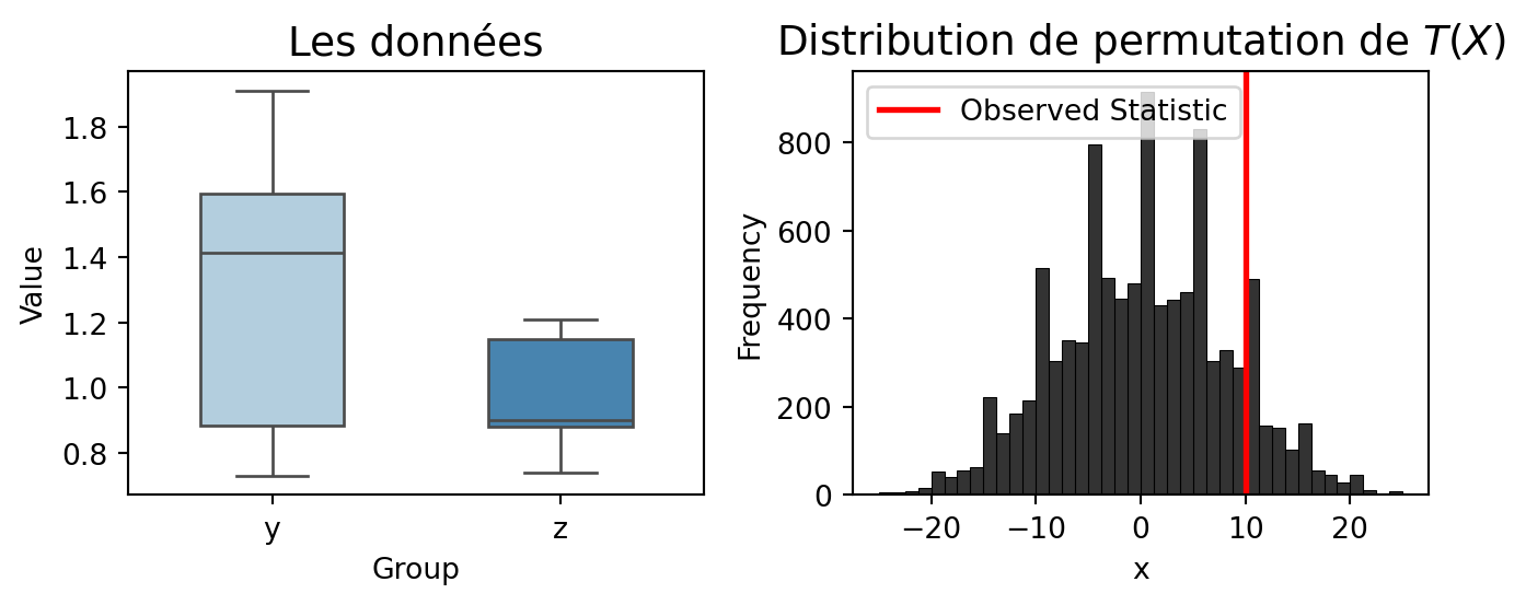
yi: placental membrane permeability at term.
zj: permeability measured between 12 and 26 weeks of gestation.

The statistic test is given by the wilcoxon statistic rank :

\[ T(X) = \sum_{i=1}^n R_i(Y) -n(N+1)/2 \]

The alternative of interest is that the placental membrane is more permeable during full-term pregnancy.

y = np.array([0.80, 0.83, 1.89, 1.04, 1.45, 1.38, 1.91, 1.64, 0.73, 1.46])
z = np.array([1.15, 0.88, 0.90, 0.74, 1.21])

# Wilcoxon statistic rank

rankwilcoxon = lambda y, z: np.sum(
    rankdata(np.concatenate([np.asarray(y), np.asarray(z)]))[:len(y)]
) - len(y) * (len(y) + len(z) + 1) / 2

res = twosamp_perm(y, z, func=rankwilcoxon, nsamp=9999, alternative="greater")

print(f"Statistic : {res['statistic']}," 
      f" p-value : {res['p-value']}")

Statistic : 10.0, p-value : 0.1265

 #--- Create Figure ---
fig, axes = plt.subplots(1, 2, figsize=(7, 3))

# --- Left Plot: Boxplot of Data ---
sns.boxplot(data=[y, z], ax=axes[0], width=0.5, palette="Blues", fliersize=3)
axes[0].set_xticks([0, 1])
axes[0].set_xticklabels(["y", "z"])
axes[0].set_title("Les données", fontsize=14)
axes[0].set_xlabel("Group")
axes[0].set_ylabel("Value")

# --- Right Plot: Permutation Distribution ---
sns.histplot(res['sample_perm'], bins=40, color="black", alpha=0.8, ax=axes[1])
axes[1].axvline(res['statistic'], color='red', linestyle='-', linewidth=2, label="Observed Statistic")
axes[1].set_title(r"Distribution de permutation de $T(X)$", fontsize=14)
axes[1].set_xlabel("x")
axes[1].set_ylabel("Frequency")
axes[1].legend()

plt.tight_layout()
plt.show()