Fourrier Transformation

Author

Jumbong Junior

Published

July 22, 2025

Introduction

When we were in our third year of the Risk Management program at an engineering school, we took a course on the calibration of stochastic processes. To assess our understanding, the instructor gave us a selection of academic papers and asked us to choose one, study it thoroughly, and reproduce its results.

We chose the paper by El Kolei (2013), which proposes a method for estimating the parameters of stochastic volatility models based on contrast minimization and deconvolution.

To do so, we had to implement an optimization algorithm that relies on the Fourier transform to evaluate the following function:

\[ \hat{f}(\nu) = \int_{-\infty}^{+\infty} f_{\theta}(t) e^{-2i\pi\nu t} dt \] où \(f_{\theta}(y) = \frac{1}{2\sqrt{\pi}} \left(\frac{-i \phi y \gamma^2 \exp\left(-\frac{y^2}{2} \gamma^2\right)}{\exp\left(-i \mathcal{E} y\right) 2^{iy} \Gamma\left(\frac{1}{2} + iy\right)}\right)\) andd \(\theta = (\phi, \gamma, \mathcal{E})\) a vector of parameters to estimate.

To compute the Fourier transform of \(f\), El Kolei (2013) uses the left Riemann sum (rectangle quadrature) method implemented in MATLAB and suggests that using the Fast Fourier Transform (FFT) algorithm could accelerate the computation of the Fourier transform.

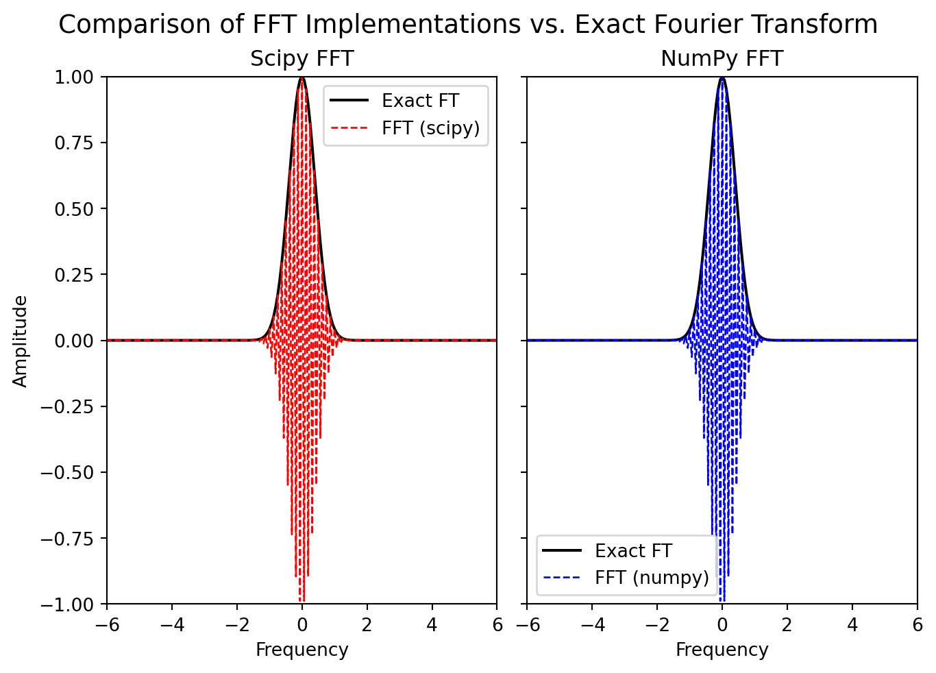
We decided to reproduce the paper using Python. Implementing the left rectangle quadrature method was straightforward, and we initially believed that the scipy.fft and numpy.fft libraries would allow us to compute the Fourier transform of \(f\) using the FFT algorithm.

However, we were surprised to discover that these functions do not compute the Fourier transform of a continuous function but rather the discrete Fourier transform (DFT) of a finite sequence. The plot below illustrates this observation.

import numpy as np
import matplotlib.pyplot as plt
from scipy.fft import fft, fftfreq, fftshift

# Define the function f(t) = exp(-pi * t^2)
def f(t):
    return np.exp(-np.pi * t**2)

# Parameters
N = 1024
T = 1.0 / 64
t = np.linspace(-N/2*T, N/2*T, N, endpoint=False)
y = f(t)

# FFT with scipy
yf_scipy = fftshift(fft(y)) * T
xf = fftshift(fftfreq(N, T))
FT_exact = np.exp(-np.pi * xf**2)

# FFT with numpy
yf_numpy = np.fft.fftshift(np.fft.fft(y)) * T
xf_numpy = np.fft.fftshift(np.fft.fftfreq(N, T))

# Plot with subplot_mosaic
fig, axs = plt.subplot_mosaic([["scipy", "numpy"]], figsize=(7, 5), layout="constrained", sharey=True)

# Scipy FFT
axs["scipy"].plot(xf, FT_exact, 'k-', linewidth=1.5, label='Exact FT')
axs["scipy"].plot(xf, np.real(yf_scipy), 'r--', linewidth=1, label='FFT (scipy)')
axs["scipy"].set_xlim(-6, 6)
axs["scipy"].set_ylim(-1, 1)
axs["scipy"].set_title("Scipy FFT")
axs["scipy"].set_xlabel("Frequency")
axs["scipy"].set_ylabel("Amplitude")
axs["scipy"].legend()
axs["scipy"].grid(False)

# NumPy FFT
axs["numpy"].plot(xf_numpy, FT_exact, 'k-', linewidth=1.5, label='Exact FT')
axs["numpy"].plot(xf_numpy, np.real(yf_numpy), 'b--', linewidth=1, label='FFT (numpy)')
axs["numpy"].set_xlim(-6, 6)
axs["numpy"].set_title("NumPy FFT")
axs["numpy"].set_xlabel("Frequency")
axs["numpy"].legend()
axs["numpy"].grid(False)

plt.suptitle("Comparison of FFT Implementations vs. Exact Fourier Transform", fontsize=14)
plt.show()

This motivation led us to write this article to explain how to compute the Fourier transform of a function using both the left Riemann sum (rectangle quadrature) method and the Fast Fourier Transform (FFT) algorithm.

The paper by El Kolei (2013) illustrates an application of the Fourier transform in finance and ecology. Beyond these domains, the Fourier transform plays a key role in spectral analysis, solving partial differential equations, evaluating integrals, and computing series sums. It is widely used in physics, engineering, and signal processing.

In the literature, several articles discuss approximating the Fourier transform and implementing it using numerical methods. However, we have not found a source as clear and comprehensive as the one by Balac (2011), which proposes a quadrature-based approach to compute the Fourier transform and explains how to use the FFT algorithm to compute the discrete Fourier transform.

We use Balac (2011) as our primary reference to show how to approximate the Fourier transform in Python using both methods: the left rectangle quadrature method and the Fast Fourier Transform (FFT) algorithm.

Definition and Properties of the Fourier Transform

We adopt the framework presented by Balac (2011) to define the Fourier transform of a function \(f\) and to introduce its properties.

The functions considered belong to the space of integrable functions, denoted \(L^1(\mathbb{R,K})\), consisting of all functions \(f:\mathbb{R} \to \mathbb{K}\) [where \(\mathbb{K}\) is either \(\mathbb{R}\) or \(\mathbb{C}\)]. These functions are integrable in the sense of Lebesgue, meaning that the integral of their absolute value is finite: \[ \int_{-\infty}^{+\infty} |f(t)| dt < +\infty. \]

So, for a function \(f\) to belong to \(L^1(\mathbb{R}, \mathbb{K})\), the product \(f(t) \cdot e^{-2i\pi\nu t}\) must also be integrable for all \(\nu \in \mathbb{R}\). In that case, the Fourier transform of \(f\), denoted \(\hat{f}\) (or sometimes \(\mathcal{F}(f)\)), is defined for all \(\nu \in \mathbb{R}\) by:

\[ \hat{f}(\nu) = \int_{-\infty}^{+\infty} f(t) \, e^{-2i\pi\nu t} \, dt. \]

The key takeaway is that the Fourier transform \(\hat{f}\) of a function \(f\) is a complex-valued, linear function that depends on the frequency \(\nu\). If \(f \in L^1(\mathbb{R})\), is real-valued and even, then \(\hat{f}\) is also real-valued and even. Conversely, if \(f\) is real-valued and odd, then \(\hat{f}\) is purely imaginary and odd as well.

For some functions, the Fourier transform can be computed analytically. For example, for the function \(f : t \in \mathbb{R} \mapsto \mathbb{1}_{[-\frac{a}{2}, \frac{a}{2}]}(t)\), the Fourier transform is given by: \[ \hat{f} : \nu \in \mathbb{R} \mapsto a sinc(a \pi \nu) \] where \(sinc(t) = \frac{\sin(t)}{t}\) is the sinc function.

However, for many functions, the Fourier transform cannot be computed analytically. In such cases, we can use numerical methods to approximate it. We will explore these numerical approaches in the following sections of this article.

How to approximate the Fourier Transform?

The Fourier transform of a function \(f\) is defined as an integral over the entire real line. However, for the functions that are integral in the sense of lebesgue and that have a practical applications tend to 0 as \(|t| \to +\infty\). And we can approximate the Fourier transform by integrating over a finite interval \([-T, T]\). If the lenght of the interval is large enough, or if the function decays quickly when t tends to infinity, this approximation will be accurate.

\[ \hat{f}(\nu) \approx \int_{-T}^{T} f(t) e^{-2i\pi\nu t} dt \]

In his article, Balac (2011) goes further by showing that approximating the Fourier transform involves three key mathematical tools:

Fourier series, in the context of a periodic signal,
The Fourier transform, for non-periodic signals,
The discrete Fourier transform, for discrete signals.

For each of these tools, computing the Fourier transform essentially comes down to evaluating the following integral: \[ \hat{f}(\nu) \approx \int_{-\frac{T}{2}}^{\frac{T}{2}} f(t) e^{-2i\pi\nu t} dt \] I recommend reading his article for more details on these three tools. Next, we will focus on the numerical computation of the Fourier transform using quadrature methods, a technique for performing numerical integration.

Numerical Computation of the Fourier Transform

We show that computing the Fourier transform of a function \(f\) consists to approximating it by the integral the following integral over the interval \([-\frac{T}{2}, \frac{T}{2}]\): \[ \underbrace{ \int_{-\infty}^{+\infty} f(t)\, e^{-2\pi i \nu t} \, dt }_{=\,\hat{f}(\nu)} \approx \underbrace{ \int_{-\frac{T}{2}}^{\frac{T}{2}} f(t)\, e^{-2\pi i \nu t} \, dt }_{=\,\tilde{S}(\nu)} \]

where T is a large enough number such that the integral converges. Une valeur approchée of the integral \(\tilde{S}(\nu) = \int_{-\frac{T}{2}}^{\frac{T}{2}} f(t)\, e^{-2\pi i \nu t} \, dt\) can be computed using quadrature methods. In the next section, we will approximate the integral using the quadrature method of rectangles à gauche.

Quadrature method of left Rectangles

To compute the integral \(\tilde{S}(\nu) = \int_{-\frac{T}{2}}^{\frac{T}{2}} f(t)\, e^{-2\pi i \nu t} \, dt\), using the quadrature method of left rectangles, we follow these steps:

Discretization of the Interval:: We divide the interval \([-\frac{T}{2}, \frac{T}{2}]\) into \(N\) uniform subintervals of length \(h_t = \frac{T}{N}\). The discretization points[eft endpoints of the rectangles] in the interval are given by:

\[ t_k = -\frac{T}{2} + k \cdot h_t, \quad k = 0, 1, \ldots, N-1. \]

Approximation of the Integral: Using the Chasles relation, we can approximate the integral \(\tilde{S}(\nu)\) as follows:

\[ \tilde{S}(\nu) = \int_{-\frac{T}{2}}^{\frac{T}{2}} f(t)\, e^{-2\pi i \nu t} \, dt = \sum_{k=0}^{N-1} \int_{t_k}^{t_{k+1}} f(t)\, e^{-2\pi i \nu t} \, dt. \]

By taking into account that we have \(t_{k+1} - t_k = h_t\), and \(t_k = -\frac{T}{2} + k \cdot h_t = T(\frac{k}{N} - \frac{1}{2})\), we can rewrite the integral as: \[ \tilde{S}(\nu) = \sum_{k=0}^{N-1} f(t_k) e^{-2\pi i \nu t_k} h_t. \]

We call it the quadrature method of left rectangles because it uses the left endpoint \(t_k\) of each subinterval to approximate the value of the function \(f(t)\) at that point.

Final Formula: The final formula for the approximation of the Fourier transform is given by:

\[ \boxed{ \forall \nu \in \mathbb{R} \quad \underbrace{ \int_{-\frac{T}{2}}^{\frac{T}{2}} f(t)\, e^{-2\pi i \nu t} \, dt }_{=\,\tilde{S}(\nu)} \approx \underbrace{ \frac{T}{n} e^{i \pi \nu T} \sum_{k=0}^{n-1} f_k\, e^{-2 i \pi \nu T k / n} }_{=\,\tilde{S}_n(\nu)} \quad \text{où } f_k = f\left( \frac{2k - n}{2n} T \right). } \]

Implementation of the left rectangle quadrature method in Python.

The function tfquad below implements the left rectangle quadrature method to compute the Fourier transform of a function f at a given frequency nu.

import numpy as np

def tfquad(f, nu, n, T):
    """
    Computes the Fourier transform of a function f at frequency nu
    using left Riemann sum quadrature over the interval [-T/2, T/2].

    Parameters:
    ----------
    f : callable
        The function to transform. Must accept a NumPy array as input.
    nu : float
        The frequency at which to evaluate the Fourier transform.
    n : int
        Number of quadrature points.
    T : float
        Width of the time window [-T/2, T/2].

    Returns:
    -------
    tfnu : complex
        Approximated value of the Fourier transform at frequency nu.
    """
    k = np.arange(n)
    t_k = (k / n - 0.5) * T
    weights = np.exp(-2j * np.pi * nu * T * k / n)
    prefactor = (T / n) * np.exp(1j * np.pi * nu * T)

    return prefactor * np.sum(f(t_k) * weights)

We can also use SciPy’s quad function to define the Fourier transform of a function f at a given frequency nu. The function tf_integral below implements this approach. It uses numerical integration to compute the Fourier transform of f over the interval \([-T/2, T/2]\).

from scipy.integrate import quad

def tf_integral(f, nu, T):
    """Compute FT of f at frequency nu over [-T/2, T/2] using scipy quad."""
    real_part = quad(lambda t: np.real(f(t) * np.exp(-2j * np.pi * nu * t)), -T/2, T/2)[0]
    imag_part = quad(lambda t: np.imag(f(t) * np.exp(-2j * np.pi * nu * t)), -T/2, T/2)[0]
    return real_part + 1j * imag_part

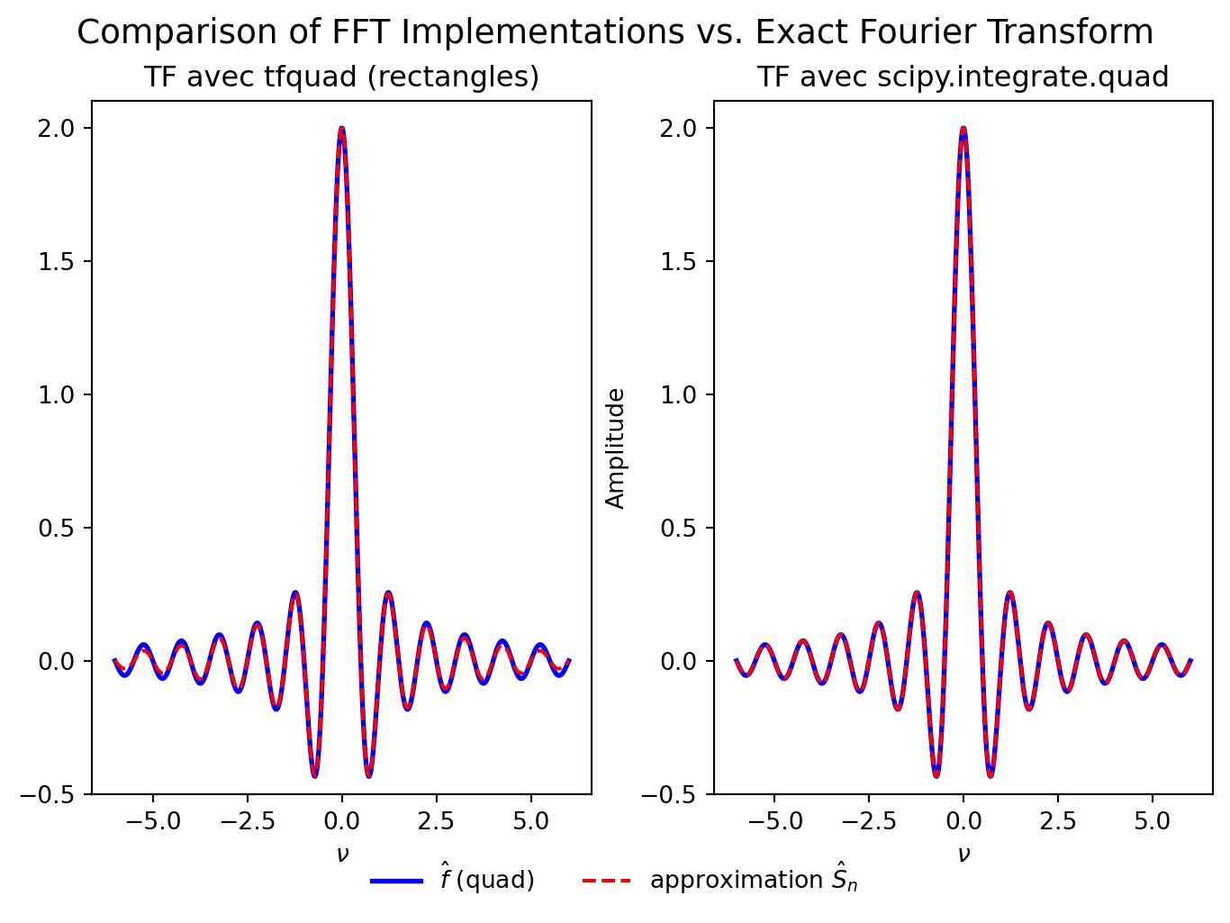
import numpy as np
import matplotlib.pyplot as plt

# ----- Function Definitions -----

def f(t):
    """Indicator function on [-1, 1]."""
    return np.where(np.abs(t) <= 1, 1.0, 0.0)

def exact_fourier_transform(nu):
    """Analytical FT of the indicator function over [-1, 1]."""
    # f̂(ν) = ∫_{-1}^{1} e^{-2πiνt} dt = 2 * sinc(2ν)
    return 2 * np.sinc(2 * nu)


# ----- Computation -----

T = 2.0
n = 32
nu_vals = np.linspace(-6, 6, 500)
exact_vals = exact_fourier_transform(nu_vals)
tfquad_vals = np.array([tfquad(f, nu, n, T) for nu in nu_vals])

# Compute the approximation using scipy integral
tf_integral_vals = np.array([tf_integral(f, nu, T) for nu in nu_vals])

fig, axs = plt.subplot_mosaic([["tfquad", "quad"]], figsize=(7, 5), layout="constrained")

# Plot using tfquad implementation
axs["tfquad"].plot(nu_vals, np.real(exact_vals), 'b-', linewidth=2, label=r'$\hat{f}$ (exact)')
axs["tfquad"].plot(nu_vals, np.real(tfquad_vals), 'r--', linewidth=1.5, label=r'approximation $\hat{S}_n$')
axs["tfquad"].set_title("TF avec tfquad (rectangles)")
axs["tfquad"].set_xlabel(r'$\nu$')
axs["tfquad"].grid(False)
axs["tfquad"].set_ylim(-0.5, 2.1)

# Plot using scipy.integrate.quad
axs["quad"].plot(nu_vals, np.real(exact_vals), 'b-', linewidth=2, label=r'$\hat{f}$ (quad)')
axs["quad"].plot(nu_vals, np.real(tf_integral_vals), 'r--', linewidth=1.5, label=r'approximation $\hat{S}_n$')
axs["quad"].set_title("TF avec scipy.integrate.quad")
axs["quad"].set_xlabel(r'$\nu$')
axs["quad"].set_ylabel('Amplitude')
axs["quad"].grid(False)
axs["quad"].set_ylim(-0.5, 2.1)



# --- Global legend below the plots ---
# Take handles from one subplot only (assumes labels are consistent)
handles, labels = axs["quad"].get_legend_handles_labels()
fig.legend(handles, labels,
           loc='lower center', bbox_to_anchor=(0.5, -0.05),
           ncol=3, frameon=False)

plt.suptitle("Comparison of FFT Implementations vs. Exact Fourier Transform", fontsize=14)
plt.subplots_adjust(bottom=0.2)  # Make room for the legend
plt.show()

/var/folders/v8/l5q0bw4s2ln17s59y7cc86rm0000gn/T/ipykernel_31663/938168490.py:30: UserWarning:

This figure was using a layout engine that is incompatible with subplots_adjust and/or tight_layout; not calling subplots_adjust.

We are now able to compute the Fourier transform of a function using the left rectangle quadrature method. Let’s take a closer look at the characteristics and limitations of this approximation.

Characterizing the approximation using the left rectangle quadrature method

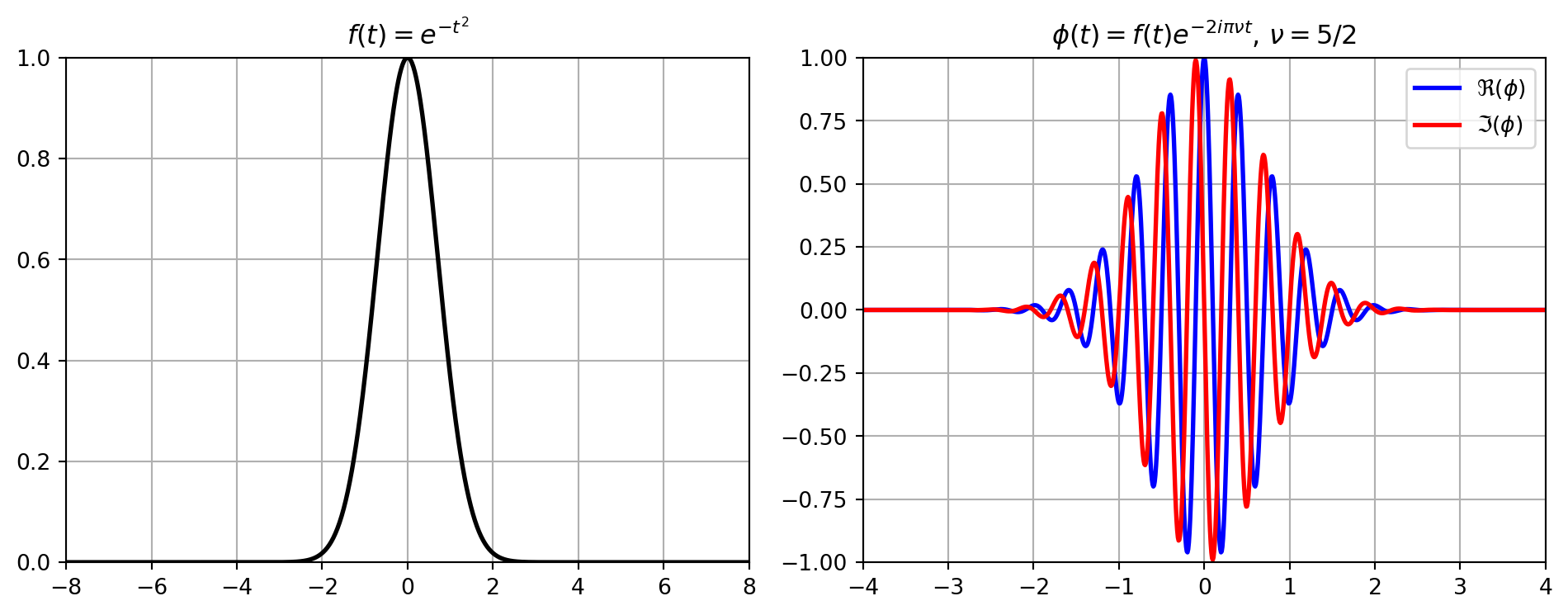
The approximation of the Fourier transform \(\hat{f}\) using the left rectangle quadrature method exhibits an oscillatory behavior by nature.

Balac (2011) highlights that the Fourier transform \(\hat{f}\) of the function \(f\) is inherently oscillatory. This behavior arises from the complex exponential term \(e^{-2\pi i \nu t}\) in the integral definition of the transform.

To illustrate this, the figure below shows the function

\[ f : t \in \mathbb{R} \mapsto e^{-t^2} \in \mathbb{R} \]

along with the real and imaginary parts of its Fourier transform

\[ \hat{f} : \nu \in \mathbb{R} \mapsto \hat{f}(\nu) \in \mathbb{C}, \]

evaluated at \(\nu = \frac{5}{2}\).

Although \(f\) is smooth, we clearly observe strong oscillations in \(\hat{f}\), highlighting the influence of the exponential kernel.

import numpy as np
import matplotlib.pyplot as plt

nu = 5 / 2
t1 = np.linspace(-8, 8, 1000)
t2 = np.linspace(-4, 4, 1000)

f = lambda t: np.exp(-t**2)
phi = lambda t: f(t) * np.exp(-2j * np.pi * nu * t)

f_vals = f(t1)
phi_vals = phi(t2)

# Plot
fig, axs = plt.subplots(1, 2, figsize=(10, 4))

axs[0].plot(t1, f_vals, 'k', linewidth=2)
axs[0].set_xlim(-8, 8)
axs[0].set_ylim(0, 1)
axs[0].set_title(r"$f(t) = e^{-t^2}$")
axs[0].grid(True)

axs[1].plot(t2, np.real(phi_vals), 'b', label=r"$\Re(\phi)$", linewidth=2)
axs[1].plot(t2, np.imag(phi_vals), 'r', label=r"$\Im(\phi)$", linewidth=2)
axs[1].set_xlim(-4, 4)
axs[1].set_ylim(-1, 1)
axs[1].set_title(r"$\phi(t) = f(t)e^{-2i\pi\nu t}$, $\nu=5/2$")
axs[1].legend()
axs[1].grid(True)

plt.tight_layout()
plt.show()

These rapid variations can create difficulties in the numerical approximation of the Fourier transform using quadrature methods, even when a large number of points \(n\) is used. One way to overcome this issue is by using the Fast Fourier Transform (FFT) algorithm.

The approximation obtained using the left rectangle quadrature method is periodic in nature.

We observe that even if the function \(f\) is not periodic, its Fourier transform approximation \(\hat{f}\) appears periodic. In fact, the function \(\hat{S}_n\), resulting from the quadrature method, is periodic with period

\[ \Delta \nu = \frac{n}{T}. \] \[ \forall \nu \in \mathbb{R} \quad \widehat{S}_n\left(\nu + \frac{n}{T} \right) = \frac{T}{n} e^{i\pi \nu T} \sum_{k=0}^{n-1} f_k \, e^{-2i\pi\left(\nu + \frac{n}{T} \right)T \frac{k}{n}} = \frac{T}{n} e^{i\pi \nu T} \sum_{k=0}^{n-1} f_k \, e^{-2i\pi \nu T \frac{k}{n}} \underbrace{e^{-2i\pi k}}_{=1} \]

\[ \phantom{\forall \nu \in \mathbb{R} \quad \widehat{S}_n\left(\nu + \frac{n}{T} \right)} = \frac{T}{n} e^{i\pi \nu T} \sum_{k=0}^{n-1} f_k \, e^{-2i\pi \nu T \frac{k}{n}} = \widehat{S}_n(\nu). \]

This periodicity of \(\hat{S}_n\) implies that it is not possible to compute the Fourier transform for all frequencies \(\nu \in \mathbb{R}\) using the quadrature method when the parameters \(T\) and \(n\) are fixed. In fact, it becomes impossible to compute \(\hat{f}(\nu)\) accurately when

\[ |\nu| \geq \nu_{\text{max}}, \]

where \(\nu_{\text{max}} = \frac{n}{T}\) is the maximum frequency that can be resolved due to the periodic nature of \(\hat{S}_n\).

As a result, in practice, to compute the Fourier transform for large frequencies, one must increase either the time window \(T\) or the number of points \(n\).

Furthermore, by evaluating the error in approximating \(\hat{f}(\nu)\) using the left rectangle quadrature method, we find that the approximation is reliable at frequency \(\nu\) when the following condition holds:

\[ |\nu| \ll \frac{n}{T} \]

\[ \frac{\nu T}{n} \ll 1. \]

Epstein (2005) shows that when using the Fast Fourier Transform (FFT) algorithm, it is possible to accurately compute the Fourier transform of a function \(f\) for all frequencies \(\nu \in \mathbb{R}\), even when \(\frac{\nu T}{n}\) is close to 1 — provided that \(f\) is piecewise continuous and has compact support.

Computing the Fourier Transform at Frequency \(\nu\) Using the FFT Algorithm.

In this section, we denote by \(\hat{S}_n(\nu)\) the approximation of the Fourier transform \(\hat{f}(\nu)\) of the function \(f\) at a point \(\nu \in \left[-\frac{\nu_{\text{max}}}{2}, \frac{\nu_{\text{max}}}{2}\right]\), where \(\nu_{\text{max}} = \frac{n}{T}\), i.e., \[ \hat{f}(\nu) \approx \hat{S}_n(\nu) = \frac{T}{n} e^{i\pi \nu T} \sum_{k=0}^{n-1} f_k\, e^{-2 i \pi \nu T k / n}. \]

We now present the Fourier transform algorithm used to approximate \(\hat{f}(\nu)\). We will not go into the details of the Fast Fourier Transform (FFT) algorithm in this article.@balac2011transformee provides a simplified explanation of the FFT, and for more in-depth technical details, we recommend the original article by Cooley and Tukey (1965).

What is important to understand is that the use of the FFT algorithm to approximate the Fourier transform of a function \(f\) is based on the result shown by Epstein (2005), which states that when \(\hat{S}_n(\nu)\) is evaluated at the frequencies \(\nu_j = \frac{j}{T}\) for \(j = 0, 1, \dots, n - 1\), it gives a good approximation of the continuous Fourier transform \(\hat{f}(\nu)\).

Moreover, \(\hat{S}_n\) is known to be periodic. This periodicity gives a symmetric role to the indices \(j \in \{0, 1, \dots, n - 1\}\) and \(k \in \{-\frac{n}{2}, -\frac{n}{2} + 1, \dots, -1\}\). In fact, the values of the Fourier transform of \(f\) over the interval \(\left[ -\frac{\nu_{\text{max}}}{2}, \frac{\nu_{\text{max}}}{2} \right]\) can be derived from the values of \(\hat{S}_n\) at the points \(\nu_j = \frac{j}{T}\), for \(j = 0, 1, \dots, n - 1\), as follows:

\[ \widehat{S}_n(\nu'_j) = \frac{T}{n} (-1)^j \sum_{k=0}^{n-1} f_k\, e^{-2i\pi j \frac{k}{n}} = \begin{cases} \widehat{S}_n(\nu_j) & \text{si } j \in \left\{0, \dots, \frac{n}{2} - 1 \right\} \\ \widehat{S}_n(\nu_{j-n}) & \text{si } j \in \left\{ \frac{n}{2}, \dots, n-1 \right\} \end{cases} \]

\[ \text{où on a exploité la relation} \quad e^{-2i\pi j \frac{k}{n}} = e^{-2i\pi (j-n) \frac{k}{n}} \times \underbrace{e^{-2i\pi k}}_{=1} = e^{-2i\pi (j-n) \frac{k}{n}} \quad \text{pour } j \in \left\{ \frac{n}{2}, \dots, n-1 \right\}. \]

This relationship shows that we can compute the Fourier transform \(\hat{S}_n\left( \frac{j}{T} \right)\) for \(j = -\frac{n}{2}, \ldots, \frac{n}{2} - 1\). Moreover, when \(n\) is a power of 2, it can be shown that the computation becomes faster (see Balac 2011). This process is known as the Fast Fourier Transform (FFT).

To summarize, we have shown that the Fourier transform of the function \(f\) can be approximated over the interval \(\left[-\frac{T}{2}, \frac{T}{2}\right]\) at the frequencies \(\nu_j = \frac{j}{T}\) for \(j = -\frac{n}{2}, \ldots, \frac{n}{2} - 1\), where \(n = 2^m\) for some integer \(m \geq 0\), by applying the FFT algorithm as follows:

Construct the finite sequence \(F\) of values \(f\left( \frac{2k - n}{2n} T \right)\) for \(k = 0, 1, \ldots, n - 1\).
Compute the discrete Fourier transform \(\hat{F}\) of the sequence \(F\) using the Fast Fourier Transform (FFT) algorithm, which is given by

\[ \hat{F}_j = \sum_{k=0}^{n-1} f_k \, e^{-2i\pi \frac{jk}{n}}, \quad \text{for } j = 0, 1, \ldots, n-1. \]
Reindex and symmetrize the values to span \(j = -\frac{n}{2}, \ldots, -1\).
Multiply each value in the array by \(\frac{T}{n} (-1)^{j-1}\), where \(j \in \{1, \ldots, n\}\).

This yields an array corresponding to the values of the Fourier transform \(\hat{f}(\nu_j)\), with \(\nu_j = \frac{j}{T}\) for \(j = -\frac{n}{2}, \ldots, \frac{n}{2} - 1\).

The following Python function tffft implements these steps to compute the Fourier transform of a given function.

import numpy as np
from scipy.fft import fft, fftshift

def tffft(f, T, n):
    """
    Calcule la transformée de Fourier approchée d'une fonction f à support dans [-T/2, T/2],
    en utilisant l’algorithme FFT.

    Paramètres
    ----------
    f : callable
        Fonction à transformer (doit être vectorisable avec numpy).
    T : float
        Largeur de la fenêtre temporelle (intervalle [-T/2, T/2]).
    n : int
        Nombre de points de discrétisation (doit être une puissance de 2 pour FFT efficace).

    Retours
    -------
    tf : np.ndarray
        Valeurs approximées de la transformée de Fourier aux fréquences discrètes.
    freq_nu : np.ndarray
        Fréquences discrètes correspondantes (de -n/(2T) à (n/2 - 1)/T).
    """
    h = T / n
    t = -0.5 * T + np.arange(n) * h  # noeuds temporels
    F = f(t)                         # échantillonnage de f
    tf = h * (-1) ** np.arange(n) * fftshift(fft(F))  # TF approximée
    freq_nu = -n / (2 * T) + np.arange(n) / T              # fréquences ν_j = j/T

    return tf, freq_nu, t

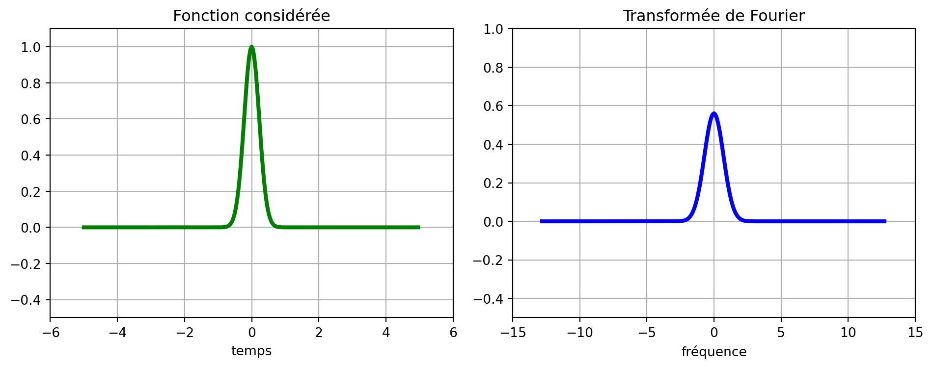
The following program illustrates how to compute the Fourier transform of the Gaussian function \(f(t) = e^{-10t^2}\) over the interval \([-10, 10]\), using the Fast Fourier Transform (FFT) algorithm.

# Paramètres
a = 10
f = lambda t: np.exp(-a * t**2)
T = 10
n = 2**8  # 256

# Calcul de la transformée de Fourier
tf, nu, t = tffft(f, T, n)

# Représentation graphique
fig, axs = plt.subplots(1, 2, figsize=(10, 4))

axs[0].plot(t, f(t), '-g', linewidth=3)
axs[0].set_xlabel("temps")
axs[0].set_title("Fonction considérée")
axs[0].set_xlim(-6, 6)
axs[0].set_ylim(-0.5, 1.1)
axs[0].grid(True)

axs[1].plot(nu, np.abs(tf), '-b', linewidth=3)
axs[1].set_xlabel("fréquence")
axs[1].set_title("Transformée de Fourier")
axs[1].set_xlim(-15, 15)
axs[1].set_ylim(-0.5, 1)
axs[1].grid(True)

plt.tight_layout()
plt.show()

The method we have just presented allows us to compute and visualize the Fourier transform of a function \(f\) at discrete points \(\nu_j = \frac{j}{T}\), for \(j = -\frac{n}{2}, \ldots, \frac{n}{2} - 1\), where \(n\) is a power of 2. These points lie within the interval \(\left[-\frac{n}{2T}, \frac{n}{2T}\right]\). However, this approach does not allow us to evaluate the Fourier transform at arbitrary points \(\nu\) in the same interval when \(\nu\) is not of the form \(\nu_j = \frac{j}{T}\).

To compute the Fourier transform of a function \(f\) at a point \(\nu\) that does not coincide with one of the sampling frequencies \(\nu_j\), interpolation methods can be used (e.g., linear, polynomial, spline interpolation, etc.). In this article, we adopt the approach proposed by Balac (2011), which relies on Shannon’s interpolation theorem to compute the Fourier transform of a function \(f\) at any point \(\nu\).

Using Shannon’s Interpolation Theorem to Compute the Fourier Transform of a Function \(f\) at a Point \(\nu\)

Que nous dit le théorème de Shannon ? Il nous dit que pour une fonction \(g\) à bande limitée c’est-à-dire dont la transformée de Fourier \(\hat{g}\) est nulle en dehors d’un intervalle \([-\frac{B}{2}, \frac{B}{2}]\), on peut reconstruire la fonction \(g\) à partir de ses échantillons \(g_k = g\left(\frac{k}{B}\right)\) pour \(k \in \mathbb{Z}\). Si on note \(\nu_c\) le plus petit réel positif tel que \(\hat{g}\) est nulle en déhors de l’intervalle \([-2 \pi \nu_c, 2 \pi \nu_c]\), alors on a la formule d’interpolation de Shannon : Pour tout \(t \in \mathbb{R}\), et \(\alpha\) un réel positif, vérifiant \(\alpha \geq \frac{1}{2 \nu_c}\), on a :

\[ g(t) = \sum_{k \in \mathbb{Z}} g(k\alpha)\, \text{sinc}\left(\frac{\pi}{\alpha}(t - k\alpha)\right) \]

où \(\text{sinc}(x) = \frac{\sin(x)}{x}\) est la fonction sinus cardinal sinc.

Balac (2011) montre que lorsque la fonction \(f\) est à support borné dans un intervalle \([-T/2, T/2]\), on peut utiliser le théorème d’interpolation de Shannon pour calculer la transformée de Fourier \(\hat{f}(\nu)\) pour tout \(\nu \in \mathbb{R}\) en utilisant les valeurs de la transformée de Fourier discrète \(\hat{S}_n(\nu_j)\) pour \(j = -\frac{n}{2}, \ldots, \frac{n}{2} - 1\). Pour ce faire, il considère \(\alpha = \frac{1}{T}\) et obtient pour tout \(\nu \in \mathbb{R}\) la formule d’interpolation de Shannon suivante : \[ \hat{f}(\nu) = \sum_{j=-\frac{n}{2}}^{\frac{n}{2}-1} \hat{S}_n\left(\frac{j}{T}\right)\, \text{sinc}\left(\pi T\left(\nu - \frac{j}{T}\right)\right) \]

Le programme ci-dessous illustre l’utilisation du théorème d’interpolation de Shannon pour calculer la transformée de Fourier d’une fonction \(f\) en un point \(\nu\).

import numpy as np

def shannon(tf, nu, T):
    """
    Approxime la valeur de la transformée de Fourier de la fonction f en la fréquence 'nu'
    à partir de ses valeurs discrètes calculées via la FFT.

    Paramètres :
    - tf : tableau numpy, valeurs de la TF (centrées avec fftshift) aux fréquences j/T pour j = -n/2, ..., n/2 - 1
    - nu : float, fréquence à laquelle on veut approximer la TF
    - T  : float, largeur de la fenêtre temporelle utilisée pour la FFT

    Retour :
    - tfnu : approximation de la TF en la fréquence 'nu'
    """
    n = len(tf)
    tfnu = 0.0
    for j in range(n):
        k = j - n // 2  # correspond à l'indice j dans {-n/2, ..., n/2 - 1}
        tfnu += tf[j] * np.sinc(T * nu - k)  # np.sinc(x) = sin(pi x)/(pi x) en numpy

    return tfnu

Enfin, nous pouvons definir la

def fourier_at_nu(f, T, n, nu):
    """
    Calcule la transformée de Fourier de f en la fréquence nu
    en utilisant tffft + interpolation de Shannon.
    """
    tf, _, _ = tffft(f, T, n)
    return shannon(tf, nu, T)

a = 0.5
f = lambda t: np.exp(-a * np.abs(t))                          # Fonction à transformer
fhat_exact = lambda nu: (2 * a) / (a**2 + 4 * np.pi**2 * nu**2)  # TF exacte

T = 40     # largeur de la fenêtre
n = 2**10  # nombre de points de discrétisation

# Calcul pour nu = 3/T
nu = 3 / T
# Valeur exacte de la TF
exact_value = fhat_exact(nu)
# Approximation de la TF en nu
approx_value = fourier_at_nu(f, T, n, nu)
print(f"Exact value at nu={nu}: {exact_value}")
print(f"Approximation at nu={nu}: {approx_value}")

# Calcul pour nu = pi/T
nu = np.pi / T
# Valeur exacte de la TF
exact_value = fhat_exact(nu)
# Approximation de la TF en nu
approx_value = fourier_at_nu(f, T, n, nu)
print(f"Exact value at nu={nu}: {exact_value}")
print(f"Approximation at nu={nu}: {approx_value}")

Exact value at nu=0.075: 2.118347413776218
Approximation at nu=0.075: (2.1185707502943534-3.313537429625715e-17j)
Exact value at nu=0.07853981633974483: 2.0262491352594427
Approximation at nu=0.07853981633974483: (2.0264201680784835-2.0283412100428305e-17j)

Une alternative à l’interpolation de Shannon est d’utiliser d’autres méthodes d’interpolation comme l’interpolation de Lagrange ou l’interpolation de Newton.

Conclusion

Balac, Stéphane. 2011. “La Transformée de Fourier Vue Sous l’angle Du Calcul Numérique.”

Cooley, James W, and John W Tukey. 1965. “An Algorithm for the Machine Calculation of Complex Fourier Series.” Mathematics of Computation 19 (90): 297–301.

El Kolei, Salima. 2013. “Parametric Estimation of Hidden Stochastic Model by Contrast Minimization and Deconvolution: Application to the Stochastic Volatility Model.” Metrika 76 (8): 1031–81.

Epstein, Charles L. 2005. “How Well Does the Finite Fourier Transform Approximate the Fourier Transform?” Communications on Pure and Applied Mathematics: A Journal Issued by the Courant Institute of Mathematical Sciences 58 (10): 1421–35.